Difference between revisions of "Tutorials:11 Manual Calibration"
(No difference)
|
Latest revision as of 18:39, 8 December 2008
This tutorial is under construction. Attempt at your own risk. The files referenced in this tutorial are not available, although any valid GSSHA™ project file and solution can be substituted.
This tutorial is compatible with:
- WMS Version 8.1
- GSSHA Version 3.0b and later
Disclaimer: GSSHA tutorial exercises do not represent real world conditions
We shall practice calibrating a simplified model. It does not have ET or long-term turned on. This data set is more to help you become familiar with the WMS interface for manually calibrating your own model than it is to end up with a calibrated model. If you have WMS running, close it and open up a new instance.
- In the 2D Grid Module, select GSSHA™ | Open Project File…
- Browse to the Finished_Tutorials/calibrate/start folder. Open the base_calib.prj file.
- Select GSSHA™ | Read Solution… Make sure that the base_calib.prj file shows up in the dialog. Hit Ok.
- Zoom in around the outlet. You’ll notice a short stream that connects the outlet to the rest of the stream network.
- In the Map Module, using the Select Feature Node tool, double-click the node at the upstream side of that short segment.
- Click on the Observations button.
- Open up Microsoft® Excel®. Open the observed.xls workbook in the Finished_tutorials\calibrate folder.
- Copy cells A2 to B202.
- In WMS, in the Observations dialog, select the drop-down box under the observed column in the upper pane. Select the Edit field.
- Paste the data into the XY Series editor. Look at the plot of the data and click OK.
- Under base_calib change hide to be show.
- Select the Calibration Analysis button.
- Select OK, OK, OK to get back to the main WMS screen.
- Select a parameter that you would like to modify and change it. (Try stream or overland roughness values to start with.)
- After creating a new folder, save the project in the new folder with a different base file name than ‘base_calib.’
- Run the model.
This is the project we shall use as the starter project. Let’s look at the data.
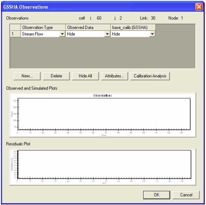
This dialog (shown in the following figure) is used to compare solution results with each other and with the observed data. Let’s load the observed data.
Notice that under the observed data column, in row 1, it says ‘Show.’ The show and hide commands alter the display of the data in the two plots in the lower part of the Observations dialog. Now let’s display our simulated data so that we can see what is happening.
The upper plot window now shows plots of the observed and predicted data. The lower plot window takes the difference between the two (the residuals) and plots it. Let’s look at how well our simulation matches the observed data.
The calibration analysis dialog computes a few objective functions for the set of residuals. Once you are done looking at the calibration analysis dialog:
Your next goal is to create a few more projects so that we can compare data.
Once you have run another model you can go back to the same feature node as before to look at what changed in the output and also compare the new output data with the old and with the observed data set.
GSSHA Tutorials
GSSHA Tutorial Download Website
