User's Manual

Preface

PREFACE

The work described in this report was authorized by Headquarters, U. S. Army Corps of Engineers (USACE). Funding for this report was provided by the Hydrologic Systems Branch, Coastal and Hydraulics Laboratory (CHL), Engineer Research and Development Center (ERDC) and the System Wide Water Resources Program (SWWRP). At the time of preparation, Mr. Earl Edris was the chief, Hydrologic Systems Branch, CHL, ERDC.

This report was prepared by Dr. Charles W. Downer, Coastal and Hydraulics Laboratory (CHL) Engineer Research and Development Center (ERDC), Dr. Fred L. Ogden, Department of Civil and Environmental Engineering, University of Connecticut, and Mr. Aaron Byrd USACE-ERDC-CHL.

This report was prepared under the general supervision of Mr. Earl Edris, Chief, Hydrologic Systems Branch, CHL, ERDC. Mr. Tom Richardson was Director of CHL. Dr. Steve Ashby (EL) was the SWWRP program manager. The report was reviewed by Dr Mark Jourdan, CH-HW and Dr Jeffery D. Jorgeson, CH-HW.

At the time of publication Dr. Jim Houston was ERDC Director.

This document and the software GSSHA are products of the Watershed Systems Group, Hydrologic Systems Branch, Coastal and Hydraulics Laboratory, Engineer Research Development Center. For more information about GSSHA, contact:

Barbara Parsons

Hydrologic Systems Branch

Coastal and Hydraulics Laboratory

Engineer Research Development Center

3909 Halls Ferry Road

Vicksburg, MS 39180

http://chl.wes.army.mil/software

This report should be cited as follows:

Downer, C. W., Ogden, F. L., and Byrd, A.R. 2008, GSSHAWIKI User’s Manual, Gridded Surface Subsurface Hydrologic Analysis Version 4.0 for WMS 8.1, ERDC Technical Report, Engineer Research and Development Center, Vicksburg, Mississippi.

---

---

 

1 - Introduction

GSSHA User's Manual

The Watershed Systems Group (WSG) within the Coastal and Hydraulics Laboratory of the US Army Engineer Research and Development Center (ERDC) supports the US Army and the US Army Corps of Engineers (USACE) in both military and civil operations through the development, modification and application of surface and sub-surface hydrologic models. The Department of Defense (DoD) is also charged with managing approximately 200,000 km² of land within the United States on military installations and flood control and river improvement projects. The WSG provides the Army with predictions of stream flow and stage, inundated areas, saturated areas, soil moistures, groundwater levels, and contaminant fate and transport. Predictions are provided for anticipated changes in weather conditions, project alternatives and land-use changes. The WSG uses a variety of models that are supported by the DoD graphical user interfaces (GUI) Watershed Modeling System (WMS) (Nelson, 2001), Groundwater Modeling System (GMS) (Jones, 2001), and Surfacewater Modeling System (SMS) (Zundel, 2001). These GUIs are commonly referred to the XMS system. The XMS interfaces support a variety of model classes, from simple lumped-parameter runoff models, to 2-D overland, and 3-D unsaturated groundwater models.

For many problems the distributed modeling approach may offer substantial potential improvement in capability compared with traditional lumped-parameter hydrologic models such as the USACE surface hydrologic model HEC-1 (USACE, 1985). The US Army, with additional support from the US Environmental Protection Agency (EPA), funded the development of the physically-based, distributed parameter, Hortonian runoff model CASC2D (Ogden and Julien, 2002; Downer et al., 2002a). Past experience with CASC2D has been favorable when the model has been properly applied, i.e. when Hortonian flow is the dominant process (Doe and Saghafian, 1992; Doe et al. 1996; Ogden et al., 2000; Senarath et al., 2000; Downer et al., 2002a). CASC2D Version 1.18b is linked with WMS Version 5.1 (BYU, 1997a; 1997b), which greatly simplifies model setup, results analysis and visualization. The WSG and the US Army no longer support the development or application of the CASC2D model. CASC2D development continues at Colorado State Univerity.

While Army experience with CASC2D has generally been favorable, there are many instances where the assumptions inherent in the CASC2D model limit its applicability (Senarath et al., 2000; Downer et al., 2002a). Figure 1 illustrates hillslope hydrology with an emphasis on the different runoff and streamflow generating processes. When saturation excess runoff, groundwater discharge to stream, exfiltration, etc., contribute significantly to the stream flow, the application of Hortonian runoff models is ill advised and can lead to erroneous results (Loague and Freeze, 1985; Loague, 1990; Grayson et al., 1992; Smith et al., 1994; Loague and Kyriakidis, 1997; Downer et al., 2002a).

1.1 History

The GSSHA model is a significant reformulation and enhancement of the CASC2D model. The CASC2D runoff model began with a two-dimensional overland flow routing algorithm developed and written in APL (A Programming Language) by Professor P.Y. Julien at Colorado State University. The overland flow routing module was converted from APL to FORTRAN by Dr. Bahram Saghafian, then at Colorado State University, with the addition of Green & Ampt infiltration and explicit diffusive-wave channel routing (Julien and Saghafian, 1991; Julien et al., 1995). The FORTRAN code was reformulated, significantly enhanced, and re-written in the C programming language by Dr. Bahram Saghafian at the U.S. Army Construction Engineering Research Laboratory (CERL). Implicit channel routing was added to CASC2D by Fred L. Ogden (Ogden, 1994), formerly at Colorado State University, then Associate Professor, Department of Civil and Environmental Engineering, University of Connecticut, Storrs, Connecticut, now Cline Distinguished Chair of Engineering, Environment and Natural Resources, Department of Civil & Architectural Engineering and Haub School of Environment and Natural Resources, University of Wyoming. This version, named r.hydro.casc2d, was part of the GRASS GIS for hydrologic simulations (Saghafian, 1993). Work began in 1995 to re-formulate CASC2D with the addition of continuous simulation capabilities, including an interface with the Watershed Modeling System (WMS) interface developed by Brigham Young University (BYU). This version, known as CASC2D for WMS, is distinguished from its predecessors by the addition of a number of new capabilities, numerous improvements and bug fixes, and a more stringent copyright. Johnson et al. (2000) added overland and channel transport to the CASC2D model.

The GSSHA model is a direct result of the dissertation work of Charles W. Downer, USACE-ERDC-CHL (Downer, 2002), and was developed from a need to simulate watersheds with runoff producing processes other than Hortonian flow. While the capability of the CASC2D model was included in GSSHA (many of the processes were taken directly from CASC2D) the continuous nature of the GSSHA model resulting in a need to develop an entirely new model. The first release of the model respresents a fully coupled surface water/groundwater simulator with sediment transport capability (Downer and Ogden, 2006). Since the original development of GSSHA, a myriad of improvements and capabilities have been added to model: coupling of the Green and Ampt with redistribution (GAR) model to the saturated groundwater (Downer et al, 2002), improved channel routing including non-orthogonal stream networks, reservoirs, detention basins and hydraulic structures (Downer et al., 2008), improved soil mositure accounting for use with GAR (Downer, 2008), constituent transport (Downer and Byrd, 2007), and coupling of constituent transport with the Nutrient Simulation Model (NSM) (Johnson and Gerald, 2007). The new features have been tested in a variety of watersheds (Downer et al., 2002, Downer 2008a, Downer 2008b, and others).

1.2 Purpose

GSSHA is intended to be a complete physics based wateshed analysis model and includes important processes related to the generation of runoff, stream routing, overland and stream sediment processes, and constituent transport. The primary purpose for the original version of GSSHA model is to correctly identify and realistically simulate the important hydrologic processes in watersheds. The model is intended to simulate different types of runoff production and determine the controlling physical processes in watersheds, i.e. infiltration excess, saturated source areas, and groundwater discharge. In addition, the model is to physically simulate soil erosion, transport and deposition, as well as constituent transport. Development of the model has been directed by the following requirements:

• model must be capable of explicitly calculating flows, stream depths, and soil moistures in a variety of hydrologic regimes and conditions including non-Hortonian watersheds;
• formulation must account for sub-surface effects on stream flow;
• numerical algorithms must be robust;
• model must conserve mass;
• model simulates soil erosion, transport, and deposition;
• model simulates contaminant transport problems;
• simulation times must be short enough to allow real-time predictions for use at DoD training facilities;
• model must be supported by the standard DoD graphical user interface (GUI) WMS;
• source code must be available to the U.S. Army without restrictions or limitations on modification or publication of results.

1.3 Differences Between GSSHA and CASC2D

---

---

 

2 - Model Formulation

GSSHA User's Manual

GSSHA is a physically-based, distributed-parameter, structured grid, hydrologic model that simulates the hydrologic response of a watershed subject to given hydrometeorological inputs. The watershed is divided into cells that comprise a uniform finite difference grid. Processes that occur before, during, and after a rainfall event are calculated for each grid cell and then the reponses from individual grid cells are integrated to produce the watershed response. Major components of the model include precipitation distribution, snowfall accumulation and melting, precipitation interception, infiltration, evapo-transpiration, surface water retention, surface runoff routing, channel flow routing, unsaturated zone modeling, saturated groundwater flow, overland sediment erosion, transport and deposition, channel routing of sediments, and constituent fate and transport on the overland and in channels.

During an event, rainfall is spatially and temporally distributed over the watershed. Rainfall may be intercepted by vegetation before reaching the land surface. Once an initial interception demand is reached, a fraction of the precipitation will reach the land surface. Upon reaching the land surface, precipitation may infiltrate due to gravity and capillary forces. Water remaining on the land surface may runoff as two dimensional (2-D) overland flow, after a specfied retention depth representing micro-topography has been reached. This water may eventually enter a stream and be routed to the watershed outlet as one dimensional (1-D) channelized flow. Between precipitation events, soil moisture accounting, evapo-transpiration (ET), and 2-D lateral groundwater flow may be occuring. When precipitation falls in the form of snowfall, the water equivalent volume remains on the land surface and is released as water according to an energy budget calculation.

On the overland flow plane sediment is detached due to rainfall impact and shear stresses due to overland flow. Sediments are routed overland along with the 2-D overland flow. Erosion and deposition continuously occurs on the overland plane as sediments are transported. Sediments may eventually be routed to the stream network where fines (silt and clay) are routed according the advection dispersion equation. Coarse materials are treated as bed load, which is computed according to Yang's method (ref).

Constituents may be assumed to within the soil column or on the land surface. In either case, constituent uptake occurs when water is ponded on the soil surface. Constituents move along in the 2-D overland flow, with reactions occuring as water moves across the watershed. Constituents may ultimately be deposisted into the stream network where they are transported according to the reactive advection dispersion equation.

2.1 Processes Simulated

GSSHA is a process-based model. Hydrologic processes that can be simulated and the methods used to approximate the processes with the GSSHA model are listed in Table 1. With the exception of channel routing, all processes and approximations in the original CASC2D model are also contained in the GSSHA model. The Preissmann channel routing routine (Cunge et al., 1980) was excluded because of known stability problems with the scheme when simulating trans-critical flows (Mesehle and Holly, 1997). Also, the upwind explicit channel routing method was replaced with a similar up-gradient explicit method.

Process	Approximation
Precipitation distribution	Thiessen polygons (nearest neighbor), Inverse distance-squared weighting
Snowfall accumulation and melting	Energy balance
Precipitation interception	Empirical 2 parameter with seasonal variance
Overland water retention	Specified depth
Infiltration	Green and Ampt (GA), Multi-layered GA, Green and Ampt with Redistribution (GAR), Richard’s equation (RE)
Overland flow routing	2-D diffusive wave Explicit, Alternating Direction Explicit (ADE), ADE Predictor-Corrector (ADEPC)
Channel routing	1-D diffusive wave – up-gradient explicit
Reservoir simulation	Inflow from overland Inflow from streams Rainfall input ET - Dingman (1995) Outlet strucuture control Variable area/volume
Evapo-transpiration	Deardorff, Penman-Monteith with seasonal canopy resistance
Soil moisture in the Vadose zone	Two layer model, RE
Lateral groundwater flow	2-D vertically averaged
Stream/groundwater interaction	Darcy’s law
Exfiltration	Darcy’s law
Overland Erosion	Rainfall Impact Rill and Gully Kilinc Richardson Engelund Hansen Shear Stress
Overland Sediment Deposition	Shield's law
Overland Sediment Routing	Transport Capacity 2-D Advection
Channel Routing of Fine Sediments	1-D Advection-Dispersion
Channel Routing of Sand	Bedload according to Yang's method
Reservoir Sources of Sediment	Overland lateral flow Stream flow
Reservoir Routing for Fines	Completely mixed reactor
Reservoir Routing for Sands	Overland sources deposit in reservoir boundary cells Stream sources deposit in reservoir bottom
Reservoir Fines Deposition	Uniform deposition over submerged overland cells Deposition according to Shield's equation
Overland Constituent Loading	Specified rainfall concentration Specified groundwater concentration Specified loading on soil surface Specified loading in top soil layer Point source loadings
Overland Constituent Uptake	First order reaction with materials on surface First order reaction with materials in top soil layer NSM reactions with top soil layer
Overland Constituent Transport	2-D Advection-Dispersion
Overland Reactions	First Order Decay NSM reactions
Channel Constituent Loading	Lateral inflow from overland Interaction with groundwater - specified groundwater concentration Point source loadings
Channel Constituent Transport	1-D Advection-Dispersion
Channel Reactions	First Order Decay NSM reactions
Reservoir Constituent Loading	Precipitation Lateral inflow from overland Interaction with groundwater - specified groundwater concentration Point source loadings
Reservoir Constituent Transport	Completely Mixed Reactor
Reservoir Reactions	First Order Decay NSM reactions

Table 1 – Processes and approximation techniques in the GSSHA model

GA – Green and Ampt (1911), GAR – Green and Ampt with Redistribution (Ogden and Saghafian, 1997), RE – Richards’ equation (1931), ADE – Alternating Direction Explicit (Downer et al., 2000), ADEPC – Alternating Direction Explicit, Predictor-Corrector (Downer et al, 2000).

2.2 Time Steps and Process Updates

In GSSHA the user specifies the overall model time step, in seconds, that the model uses to loop through the processes, check update times, and update processes. To avoid missing updates of processes, such as rainfall, that may be specified at 1 minute intervals, the overall model time step should be integer divisible into 60 seconds or an integer multiple of 60 s (i.e. 5,10,15,20,30,60,120,180,300). Time steps such as 7,9,13,16,21,45,90,270 should not be used, as they may result in unexpected internal model behavior. The model time step also must not be greater than the finest resolution of inputs, such as rainfall. Typical time steps for GSSHA range from 10 to 300 seconds. Smaller time steps may be required for particularly difficult problems.

The computational time step is an important parameter affecting the performance of GSSHA. In addition to setting the pace of the model, the overall model time step is used to set or initialize the temporal discretizations of many model processes. While many processes, such as channel routing, saturated and unsaturated groundwater flow, have internal model stability checks, some methods of overland flow routing do not. If the time step is too large the program may crash or produce inaccurate results. Very small time steps result in inordinately long simulation times. The best way to determine the most efficient time step is through a temporal convergence study, where the time step is varied and the model behavior is observed. This allows the user to determine the maximum time step that can be used with acceptable accuracy. As the time step is increased, the outlet hydrograph will begin to shift in position in relation to simulations with smaller time steps. As the time step is further increased, the discharge at the outlet will oscillate; further increases in the computational time-step will result in program crashes. Results of a temporal convergence study, featuring hydrograph shifting, oscillations, and model crash, are shown in Figure 4.

The appropriate time step strongly depends on watershed and rainfall characteristics. In general, shorter time steps must be used for:

• higher intensity storms,
• finer horizontal grid resolution (grid spacing),
• steeper watershed slopes,
• larger watershed areas, and
• smoother surfaces.

Shorter time steps must be used when backwater effects are generated in flat areas in the digital elevation model (DEM). If the time step is too long for any particular simulation the surface water depth in very flat areas may develop a checkerboard pattern due to oscillations in the water surface level. This eventually results in a crash. If this occurs the time step should be decreased and the simulation repeated.

At the time of this publication, only the time step for the saturated groundwater flow is specified in addition to the overall time step. The ET time step is fixed at 1 hr, the usual interval of hydrometeorological data available. To maintain stability the time step may be reduced internally for the explicit channel routing code, the unsaturated zone RE solver, the groundwater solver, and the explicit and ADE solutions for overland flow. Internal time step limitations in the model are described under the appropriate process sections. Rainfall updates are specified in the rainfall gage file and the interval between updates can vary as needed. Thus the overall time step is limited by:

1. stability issues in the overland flow scheme,
2. the smallest rainfall interval,
3. the groundwater time step, and
4. the need to be integer divisible into the groundwater time step and the smallest rainfall interval.

Timesteps for sediment and constituent fate and transport are based on the underlying hydrologic proecesses and do not have to be specified.

Guidance for time steps is shown in Table 2.

PROCESS	TYPICAL TIME STEP	DEPENDENCE	STABILITY CRITERIA
Overall model	1s- 5 min	Overland flow scheme Rainfall interval Groundwater time step
ET	1 hr	Available hydrometeorological data
Rainfall	1 min - 1 d	Available rainfall data
Interception	1 min - 1 d	Rainfall interval
GA Infiltration	1s - 5 min	Same as overland flow scheme
GA with Redistribution	1s - 5 min	Same as overland flow scheme
RE Infiltration	1s - 1 hr	Dependent on change in water content (d/dt)	0.0025<d/dt<0.025 Set by user
Overland flow routing	1s - 5 min	Stability of overland flow scheme
Explicit channel routing	1s - 1 hr	Must be equal to or less than overland flow routing time step during runoff Equal to groundwater time step when groundwater discharge only	Courant number less than 1/6
Saturated groundwater flow	10 min - 1 d	Equal to overland flow time step during runoff Must maintain channel stability during discharge to stream	Maximum number of cells added or subtracted from unsaturated zone

Table 2 – Recommended time-steps and stability criteria used in the GSSHA model

File:Figure 4.jpg

Figure 4 – Example of temporal convergence study with hydrograph shifting at 150 s time step, oscillations at 180 s, and oscillations leading to a crash at 210 s.

2.3 Inputs

GSSHA is a distributed-parameter, process-based model that requires the user to select the processes to be simulated and then provide the model with the data necessary to drive the selected options. Three types of input data are used. An ASCII text project file is used to provide the basic project information, select processes to be simulated, assign simulation parameters, and locate data files, tables and maps. Spatially distributed parameters can be assigned with maps of ASCII gridded data with a parameter value in each grid cell, with index maps and tables of parameter values that relate to the index maps, or with uniform values in every cell. Typically the data required to assign parameter values in every cell is not available. Standard practice in the application of GSSHA has been to develop index maps based on available data sources of land use, soil type, and vegetation. Typically these maps are combined to create a master land use/soil type/vegetation index map that can be used to assign all parameter values.

Parameters for each index map are then assigned using tables that reference the values in the index maps. A detailed description of using the index maps and Mapping Tables to build a GSSHA model is provided in Section 11. If available, the detailed maps containing parameter values in each cell, as described in Ogden (2000), may be input in lieu of the index maps and table.

Since distributed parameters may be assigned with a single uniform value in the project file, a table value linked to an index map, or with an ASCII map with a parameter value for every grid cell the model has been developed to prioritize parameter specification. While internally assigning parameter values the GSSHA model looks for the most detailed information first, GRASS ASCII maps, the second most detailed information second, table values linked to index maps, and finally a single uniform value from the project file. Once data from one of these sources is located, the search ends and the parameter values are assigned inside the GSSHA model. While this rule is generally applicable it is prudent not to specify multiple sources of the same parameter value in the project file. This avoids possible confusion and improper assignment of parameter values.

The Watershed Modeling System (WMS) interface, developed at the Environmental Modeling Research Laboratory (EMRL) at Brigham Young University, is recommended for developing input files and viewing output from the GSSHA model. The WMS produces GSSHA specific files from general Geographic Information System (GIS) data. WMS does not replace the functions of a GIS, though it can accept information in a variety of GIS formats. GSSHA relies on the GRASS ASCII data file format for storing spatially distributed data. The GRASS GIS is very helpful in the preparation of GSSHA data sets. Users of ARC/INFO and ARCVIEW can export data to GSSHA through the WMS interface. For more information about WMS, DoD and EPA personnel should contact:

XMS Model Support

Hydrologic Systems Branch

Coastal and Hydraulics Laboratory

Engineer Research Development Center

3909 Halls Ferry Road

Vicksburg, MS, 39180

(601) 634-4286

http://chl.wes.army.mil/software

Other users seeking information about WMS, should contact:

Aquaveo

3210 N Canyon Road

Provo, Utah 84604

801-691-5530

http://www.aquaveo.com/technical-support

email: support@aquaveo.com

---

---

 

3 - Project File

GSSHA User's Manual

GSSHA simulations require a project file that contains command line instructions or “cards” which pass options to GSSHA for a particular simulation. The name of the project file is given at run time as a command line argument for GSSHA. The following section presents all project file cards followed by a brief description of each. The project file consists of a single card on each line, followed by its argument, if any. While some cards require no argument, others require values, character strings, file names, table names, or map names. Tables are files that contain ASCII input data in a tabular format. A map name is simply the name of a floating point GRASS ASCII file that contains raster data. An index map refers to a similar file that contains integers indexed to tabular values. Throughout the manual, project card names will be presented in BOLD CAPITAL letters; arguments appear as CAPITAL ITALICS.

The project file cards may appear in the project file in any order, except the first card must be GSSHAPROJECT. Extraneous or misspelled cards are ignored. A card may be commented out by preceding the card with a pound sign (hash mark) “#”. When using the Mapping Table to assign parameter values for any process, the MAPPING_TABLE card is used. For project cards related to input parameters the units, if any, of the input argument are presented. For optional inputs, the default value, if any, is also presented.

3.1 Required Inputs

The following table lists all required project file card, which must be present in a project file. In addition to these cards, a method of assigning rainfall and overland roughness values must also be selected from the choices below.

Card	Argument	Description
GSSHAPROJECT	none	This card must appear first in the project file
GRIDSIZE ##.##	real	The size of the square model grid cells (m) (cells will be GRIDSIZExGRIDSIZE.
ROWS ##	integer	Number of rows in each raster map.
COLS ##	integer	Number of columns in each raster map.
TOT_TIME ##	integer	Total duration of the event simulation in minutes. Not required if LONG_TERM is specified.
TIMESTEP ##	real	Overall model time step (s).
OUTSLOPE ##.##	real	Slope of the cell containing the watershed outlet. Must be positive. Not required if DIFFUSIVE_WAVE is specified.
OUTROW ##	integer	The raster row where the catchment outlet is located. Not required if DIFFUSIVE_WAVE is specified.
OUTCOL ##	integer	The raster column where the catchment outlet is located. Not required if DIFFUSIVE_WAVE is specified.
ELEVATION ##.##	map name	Name of GRASS ASCII map containing watershed elevations (m).
WATERSHED_MASK "filename.msk"	map name	Name of GRASS ASCII map containing the watershed shape. Cells marked with 1 lie inside the watershed, while cells marked with a 0 lie outside. Must be the first card after GSSHAPROJECT when using GSSHATM with WMS.
HYD_FREQ ##	integer	Time (minutes) that points are written to the output hydrograph file(s).
SUMMARY "filename.sum"	file name	Output file summarizing information on options selected, inputs read, simulation results, mass conservation, and warnings generated during the simulation.
OUTLET_HYDRO "filename.otl"	file name	Output file containing time series discharge at the catchment outlet. (m3 s-1 default or, ft3 s-1 if QOUT_CFS card specified)

3.2 Mapping Table – Optional

When using the Mapping Table to assign any of the distributed parameters the Mapping Table card must be included.

Card	Argument	Description
MAPPING_TABLE "filename.cmt"	filename	Input ASCII file that assigns grid-based parameter values based on grid index maps.
ST_MAPPING_TABLE "filename.smt"	filename	Input ASCII file that assigns link/node parameter values based on stream index maps.

3.3 Overland Flow – Required

3.3.1 Required Inputs

Overland roughness coefficients must be assigned to every cell in the active grid. Overland roughness coefficients may be assigned as either a single uniform value, from a GRASS ASCII grid map, or from the Mapping Table. Only one option should be selected. Do not specify either of these cards if roughness values are to be read from the Mapping Table file.

Card	Argument	Units	Description
MANNING_N ##.##	real	none	Constant value of Manning’s roughness coefficient to be applied to the entire watershed. Mutually exclusive with ROUGHNESS and Mapping Table file assignment.
ROUGHNESS "filename.ext"	map name		Name of GRASS ASCII map containing spatially-varied overland flow Manning’s n values. Mutually exclusive with MANNING_N and Mapping Table file assignment.

3.3.2 Optional Inputs

The user can select the overland flow routing scheme. An overland retention depth may also be specified at the discretion of the user. Retention depth can be assigned as a single uniform value, from the Mapping Table, or from a GRASS ASCII grid map. Only one option should be specified.

Card	Argument	Units	Default Value	Description
OVERTYPE [type]	character		ADE	Overland routing scheme, one of: EXPLICIT, ADE, or ADE-PC
RETEN_DEPTH ["filename.ext"]	map name or none			Specifies distributed retention depth (mm) over the watershed. If followed by a map name, the file will be read in as the retention depth map. If no input is specified, then the retention depth map is generated from the Mapping Table file. Mutually exclusive with RETENTION.
RETENTION ##.##	real	mm	0.0	Specifies the uniform retention depth to be used for all overland flow cells. Mutually exclusive with RETEN_DEPTH.
READ_OV_HOTSTART "filename.ext"	map name			Name of map that specifies initial depths, m, of every overland flow cell
WRITE_OV_HOTSTART "filename.ext"	map name			Name of map that specifies overland depths at the end of the simulation, m, of every overland flow cell
OV_BOUNDARY	none			Run with overland boundary conditions turned on. The boundary conditions are specified in the mapping table.
INIT_ELEV_HEAD ##.##	real	m	0.0	Specifies an initial water surface (meters above sea level.) Used when starting models adjacent to the ocean in conjunction with overland boundary conditions.
OVERLAND_MOMENTUM	real		0.2	Use the momentum formulation from Bates et al. (2010) to compute overland flow. For versions 7.14 and higher specify the time step limitation coefficient (between 0.0 and 1.0) with this card as well. The default time step coefficient is 0.2. Higher values increase speed. Lower values increase stability.
OVERLAND_STRICT_DT	none		No	Use a strict application of the overland flow time step from Bates et al. (2010).

To include wetlands, which are optional, simply set up a wetlands table. The wetlands are turned on if the table is present and has a valid index map associated with it.

3.4 Interception – Optional

Interceptions parameters may be assigned using the Mapping Table, or by assigning GRASS ASCII maps.

Card	Argument	Description
INTERCEPTION		Do interception using data present in the Mapping Table file.
STORAGE_CAPACITY "filename.ext"	map name	Name of GRASS ASCII map containing values of the initial interception abstraction (mm). Mutually exclusive with Mapping Table file assignment.
INTERCEPTION_COEFF "filename.ext"	map name	Name of GRASS ASCII map containing values of the interception coefficient. Mutually exclusive with Mapping Table file assignment.

3.5 Rainfall Input and Options – Required

The following table lists all project file cards pertaining to rainfall input. Either, but not both, PRECIP_UNIF or PRECIP_FILE must be included in each GSSHA project file.

Card	Argument	Units	Description
PRECIP_UNIF	none		Specifies spatially and temporally uniform rainfall. Also requires: RAIN_INTENSITY, RAIN_DURATION, START_DATE, START TIME. Mutually exclusive with PRECIP_FILE.
RAIN_INTENSITY ##.##	real	mm/hr	Intensity of spatially- and temporally-uniform rainfall. Required only for PRECIP_UNIF.
RAIN_DURATION ##	integer	minutes	Duration of spatially- and temporally-uniform rainfall. Required only for PRECIP_UNIF.
START_DATE [yr mo day]	integers	year month day	Year, month, and day of the beginning of a simulation. Required only for PRECIP_UNIF. See section on rainfall input for format description. This card can also be used with long term simulations to start the simulation at a point other than the beginning of the hmet time series. See long term simulation information.
START_TIME [hr min]	integers	hr minute	Hour and minute of the beginning of a simulation. Required only for PRECIP_UNIF. See section on rainfall input for format description. This card can also be used with long term simulations to start the simulation at a point other than the beginning of the hmet time series. See long term simulation information.
PRECIP_FILE "filename.gag"	file name		Input ASCII file containing spatially and temporally varied rainfall rates (mm hr-1). See the manual section titled Precipitation Input for a description of the file format. Mutally exclusive with PRECIP_UNIF.
RAIN_INV_DISTANCE	none		Inverse distance squared rainfall interpolation. REQUIRED for PRECIP_FILE. Mutually exclusive with RAIN_THIESSEN.
RAIN_THIESSEN	none		Thiessen polygon (nearest neighbor) rainfall interpolation. Recommended particularly when rainfall rates are derived from radar estimates. REQUIRED for PRECIP_FILE. Mutually exclusive with RAIN_INV_DISTANCE.

3.6 Infiltration – Optional

Infiltration may be calculated using four different infiltration options. Green and Ampt (GA) (Green and Ampt, 1911), a multi-layered Green and Ampt Model, Green and Ampt with Redistribution (GAR) (Ogden and Saghafian, 1995), and Richards’ equation (RE) (Richards, 1931). Only one of these four methods should be selected.

Card	Argument	Description
GREEN_AMPT	none	Specifies Green and Ampt (GA) infiltration calculations.
INF_REDIST	none	Specifies Green and Ampt with Redistribution (GAR) infiltration calculations.
INF_LAYERED_SOIL	none	Specifies three layered Green and Ampt infiltration.
INF_RICHARDS	none	Specifies Richards’ Equation be used for infiltration.

3.6.1 Green and Ampt (GA)

When GREEN_AMPT is selected, values of hydraulic conductivity, wetting front suction head, porosity, and initial moisture are required. Parameter values may be input using the Mapping Table file or with the series of GRASS ASCII maps using the cards below.

Card	Argument	Description
CONDUCTIVITY "filename.ext"	map name	Name of GRASS ASCII map containing spatially varied values of soil saturated hydraulic conductivity (cm hr-1). REQUIRED for GREEN_AMPT or INF_REDIST. Mutually exclusive with Mapping Table file assignment.
CAPILLARY "filename.ext"	map name	Name of GRASS ASCII map containing spatially varied values of Green & Ampt wetting front capillary head parameter (cm). REQUIRED for GREEN_AMPT or INF_REDIST. Mutually exclusive with Mapping Table file assignment.
POROSITY "filename.ext"	map name	Name of GRASS ASCII map containing spatially varied values of soil porosity. REQUIRED for GREEN_AMPT or INF_REDIST. Mutually exclusive with Mapping Table file assignment.
MOISTURE [value]	map name or none	Used to assign the initial soil moisture content. If followed by a filename, the file will be read in as a GRASS ASCII initial soil volumetric water content map. If no input is specified, then the initial soil volumetric water content s will be input using the Mapping Table file. REQUIRED for GREEN_AMP or INF_REDIST.

3.6.2 Green and Ampt with Redistribution (GAR)

When GAR is specified, the GA parameters plus two additional parameters must be provided: the pore-distribution index, and residual saturation. These may be input in the Mapping Table file or by providing two GRASS ASCII maps using the cards below.

Card	Argument	Description
PORE_INDEX "filename.ext"	map name	Name of GRASS ASCII map containing spatially varied values of the Brooks & Corey (1964) pore-distribution index. REQUIRED for INF_REDIST. Mutually exclusive with Mapping Table file assignment.
RESIDUAL_SAT "filename.ext"	map name	Name of GRASS ASCII map containing spatially varied values of the volumetric water content of the soil at residual saturation. REQUIRED for INF_REDIST. Mutually exclusive with Mapping Table file assignment.
FIELD_CAPACITY "filename.ext"	map name	Name of GRASS ASCII map containing spatially varied values of the volumetric water content of the soil when gravity drainage ceases. REQUIRED for INF_REDIST. Mutually exclusive with Mapping Table file assignment.

3.6.3 Multi-layered Green and Ampt

The multi-layered GA parameters are assigned with the table described in Section 11, and referenced to an index map. The required project cards are listed below.

Card	Argument	Description
SOIL_TYPE_MAP "filename.ext"	index map file name	Name of GRASS ASCII map containing index numbers related to soil type.
SOIL_LAYER_INPUT_FILE "filename.ext"	file name	Input ASCII file containing values GA parameter in three soil layers for each soil referenced to in the SOIL_TYPE_MAP.

3.6.4 Richards’ Equation

When INF_RICHARDS is selected additional cards are required. There are also a number of optional input and output cards, as described below. Richard' Equation parameters may be specified in the MAPPING_TABLE, as well as in separate ASCII files.

3.6.4.1 Required Inputs

Card	Argument	Description
INF_RICHARDS	none	Specify Richards’ equation for calculation of soil moisture, infiltration, and ET if doing LONG_TERM simulations.
RICHARDS_C_OPTION [value]	character string	Type of water-content/head curve and hydraulic conductivity/head curve. BROOKS - Brooks and Corey (1964), as extended by Hutson and Cass (1987), into the wet profile; or, HAVERCAMP – Havercamp (1977) as modified by Lappala (1985).

3.6.4.2 Parameter Assignment - Required

Select either SOIL_TYPE_MAP and SOIL_LAYER_INPUT_FILE or use the Mapping Table.

Card	Argument	Description
SOIL_LAYER_INPUT_FILE "filename.ext"	file name	Input ASCII file with soil layer input parameters. Not used with MAPPING_TABLE
SOIL_TYPE_MAP "filename.ext"	index map file name	Name of GRASS ASCII map of soil type integer values corresponding to SOIL_LAYER_INPUT_FILE. Not used with MAPPING_TABLE

3.6.4.3 Optional Inputs

Card	Argument	Default	Description
WATER_TABLE "filename.ext"	map name	no water table	Simulate effect of water table on soil moisture. Specify filename of GRASS ASCII map that contains starting elevations of water table (m).
AQUIFER_DELTA_Z ##.##	real	none	Size of unsaturated cell to use in all cells below the soil column specified in the SOIL_LAYER_INPUT_FILE or Mapping Table (m).
SEASONAL_RS	none	no seasonal canopy resistance (when card is absent)	Vary the vegetation canopy resistance during the year.
RICHARDS_UPPER_OPTION [value]	character string	NORMAL	Method used to calculate hydraulic conductivity at ground surface under ponded conditions: NORMAL – from cell-centered water content of first cell, GREEN_AMPT - saturated hydraulic conductivity (Ks) of cell 1 AVERAGE - average of Ks and NORMAL
GW_ASSIGN_THETA	none	do not assign initial theta assume equilibrium values	Assign soil moisture from the file specified in the SOIL_LAYER_INPUT_FILE card, if simulating the water table.
RICHARDS_ITER_MAX ##	integer	1	Maximum number of iterations on non-linear coefficients.
RICHARDS_WEIGHT ##.##	real	1.0	Weight on inter-cell hydraulic conductivities: 1.0 - forward 0.5 - centered 0.0 - backwards
RICHARDS_K_OPTION [value]	character string	ARITHMETIC	Averaging method for inter-cell hydraulic conductivities, GEOMETRIC or ARITHMETIC
RICHARDS_DTHETA_MAX ##.##	real	0.025	Maximum allowable water content change during a time-step.

3.6.4.4 Optional Output

Card	Argument	Description
IN_THETA_LOCATION "filename.ext"	file name	Input ASCII file that contains locations (row col) of cells to output time series moisture data. Works with all infiltration types GREEN_AMPT INF_REDIST INF_LAYERED_SOIL INF_RICHARDS. Output is time series of soil moisture for each location. Output is time series of soil moisture every HYD_FREQ minutes. The exact output varies with model setup. The first line in the file should be the number of locations followed by one (row col) pair for each location desired. For example, if you wanted output from 3 locations: row 1 col 1, row 10, col 9, and row 100 col 90, your input file would look like: 3 1 1 10 9 100 90
OUT_THETA_LOCATION "filename.ext"	file name	Filename to output time series moisture data every HYD_FREQ minutes at cells specified in IN_THETA_LOCATION. Output is listed in same order as input. Output is time series of soil moisture for each location. If doing LONG_TERM simulations, output is time series of soil moisture for each soil layer in your soil moisture model. The number of layers is dependent on how you have set up your soils. Output will be listed in the same order as the inputs. There will be one column for each soil layer for each output location. For INF_REDIST and INF_LAYERED_SOIL there will be two columns for each location. If there is only one soil layer in your model, then the second column for each location will have a no data card, -999.99. If you are simulating groundwater and the groundwater overtakes a layer at a location, the soil moisture will remain at saturation while that layer at that location is under the groundwater. If you are not doing long term simulations, only the surface soil moisture is listed, so only one column per location. If simulating INF_RICHARDS then there is output for every RE cell in the soil column for each output location. As the number of cells in the RE solution can vary both spatially and temporally (when simulating groundwater), the number of output columns can vary over time. For this reason, results from RE may be most useable if output only one location at a time.

3.6.7 Special Infiltration Cards

Card	Argument	Description
READ_SM_HOTSTART "filename.ext"	file name	Input GRASS ASCII map file that contains starting surface soil moistures specified for every grid cell in the watershed. Works with all infiltration options.
WRITE_SM_HOTSTART "filename.ext"	file name	Filename to output GRASS ASCII map of soil moistures for every grid cell in the watershed at the end of the simulation. Works with all infiltration options.

3.7 Channel Routing – Optional

3.7.1 Required Inputs

The following cards are REQUIRED for the simulation of channel routing.

Card	Argument	Description
DIFFUSIVE_WAVE	none	Specifies explicit diffusive-wave 1-D channel routing.
CHAN_EXPLIC	none	Specifies explicit diffusive-wave 1-D channel routing. Performs same function as DIFFUSIVE_WAVE.
CHANNEL_INPUT "filename.cif"	file name	Input ASCII file containing channel network connectivity and cross-sectional information for each link/node.
STREAM_CELL "filename.gst"	file name	Input ASCII file containing channel/grid connectivity information.
OUTLET_HYDRO "filename.otl"	file name	Output ASCII file containing discharge (m3 s-1) unless QOUT_CFS flag is specified (ft3 s-1)
SECTION_TABLE "filename.ext"	file name	Input ASCII file containing cross-section information for irregular, break-point channel cross-sections. REQUIRED if look-up table cross-sections are specified in the CHANNEL_INPUT file.

3.7.2 Initial Condition and Boundary Condition - Optional

Card	Argument	Description
EXPLIC_BACKWATER "filename.ext"	file name	Save explicit channel routing end of run values of channel depth (m) and discharge (m3 s-1) for each cell.
EXPLIC_HOTSTART "filename.ext"	file name	Start explicit channel calculations using the values of channel depth and flow in the named file.
WRITE_CHAN_HOTSTART "filename"	file name	Save explicit channel routing end of run values of channel depth (m) and discharge (m3 s-1) for each cell. Depths and discharges will be saved in separate files. Depths will be saved in a file with name "filename" with extension .dht. Discharges will be saved in a file with name "filename" with extension .qht.
READ_CHAN_HOTSTART "filename"	file name	Start explicit channel calculations using the values of channel depth and flow in the named file. Depths should be in a file with the name "filename" with extension .dht. Discharges should be in a file with the name "filename" and with extension .qht.
OVERBANK_FLOW	none	Allow water in channel to flow back onto overland flow plane when stream elevation is above top of bank and the adjacent overland cell elevation.
OVERBANK_MAX_DV	float	Fraction of stream water above TOB that can exit the channel during a single time step when the OVERBANK_FLOW card is specified. Defualt value is 0.01.
OVERLAND_BACKWATER	none	Include backwater effects on overland when stream water surface elevation or TOB is greater than overland flow surface elevation without allowing water in channel to flow back onto overland.
CHAN_POINT_INPUT	file name	Input ASCII file containing the point source input location, discharge, and concentrations.
MAX_COURANT_NUMBER	float	Value to limit maximum fractional change in channel volume for stability. Default is 0.04.
HEAD_BOUND	none	Specified head boundary at the channel outlet. Requires BOUND_DEPTH or BOUND_TS card.
BOUND_DEPTH	float	Specified static head boundary at the channel outlet (m). Used with HEAD_BOUND card, exclusive to BOUND_TS card.
BOUND_TS	time series name	Name of the time series used for the specified channel boundary in the TIME_SERIES_FILE. Used with HEAD_BOUND card, exclusive to BOUND_DEPTH card.
CHANNEL_MOMENTUM	float	Use the momentum formulation for channel flow in version 7.14 and higher. The value specified is the time step limitation coefficient, between the value of 0.0 and 1.0. Higher values increase speed. Lower values increase stability. The default value is 0.2.

3.7.3 Stream Losses/Gains - Optional

3.7.3.1 General

Card	Argument	Units	Description
STREAM_LOSS	none	none	Card is used to specify that stream losses be computed when the WATER_TABLE card is not included in the project file.

3.7.3.2 Parameters

Used with WATER_TABLE or STREAM_LOSS card. These parameters may also be distributed along the channel by assigning in the CHAN_INPUT file.

Card	Argument	Units	Description
K_RIVER ##.##	real	cm hr-1	Uniform hydraulic conductivity of streambed material. REQUIRES WATER_TABLE or STREAM_LOSS. May also be distributed in CHAN_INPUT file.
M_RIVER ##.##	real	cm	Uniform thickness of streambed material. Requires WATER_TABLE or STREAM_LOSS. May also be distributed in CHAN_INPUT file.

3.7.4 Optional Output

Card	Argument	Description
IN_HYD_LOCATION "filename.ihl"	table name	Input ASCII file specifying link/node pairs to write out time series data specified by OUT_HYD_LOCATION, OUT_DEP_LOCATION, or OUT_CON_LOCATION.
OUT_HYD_LOCATION "filename.ohl"	filename	Filename to output time series discharge data (m3 s-1 or ft3 s-1) at points specified in IN_HYD_LOCATION. REQUIRED if IN_HYD_LOCATION was specified.
OUT_DEP_LOCATION "filename.odl"	filename	Filename to output channel depths (m) every HYD_FREQ time steps at locations specified in the IN_HYD_LOCATION file.
IN_SED_LOC "filename.isl"	table name	Input ASCII file containing a list of internal link/node locations where the user wants to save sediment hydrographs. Format identical to IN_HYD_LOC option. REQUIRES SOIL_EROSION.
OUT_SED_LOC "filename.osl"	filename	Filename to output sediment flux hydrographs every HYD_FREQ time steps at internal catchment locations specified in the IN_SED_LOC file. REQUIRED if SOIL_EROSION and IN_SED_LOC card are specified.
IN_GWFLUX_LOCATION "filename.igf"	table name	Input ASCII file specifying link/node pairs to write out time series of stream/groundwater exchange flux in the file OUT_GWFLUX_LOCATION.
OUT_HYD_LOCATION "filename.ogf"	filename	Filename to output time series stream/groundwater exchange flux data (m2 s-1 or ft3 s-1) at points specified in IN_GWFLUX_LOCATION. REQUIRED if IN_GWFLUX_LOCATION was specified.
STRICT_JULIAN_DATE	none	Specifies all time series data use strict Julian format.
CHAN_DEPTH "filename.cdp"	filename	Filename to output link/node data of channel depth (m) every MAP_FREQ time steps.
CHAN_STAGE "filename.cds"	filename	Filename to output link/node data of channel stage (m) every MAP_FREQ time steps.
CHAN_DISCHARGE "filename.cdq"	filename	Filename to output link/node data of channel discharge (m3 s-1) every MAP_FREQ time steps.
CHAN_VELOCITY "filename.cdv"	filename	Filename to output link/node data of channel velocity (m s-1) every MAP_FREQ time steps.
LAKE_OUTPUT "filename.lel"	filename	Filename to output reservoir elevation (m) and volume (m3) for each reservoir in the order listed in the .cif file every MAP_FREQ time steps.

3.8 Continuous Simulations – Optional

Continuous simulations require general information about the watershed location, selection of a method to calculate evapo-transpiration (ET), hydrometeorological (HMET) data in one of three available formats, and the appropriate distributed data either from the Mapping Table file or from GRASS ASCII maps.

3.8.1 Required Inputs

Card	Argument	Units	Description
LONG_TERM	none		Specifies continuous simulation. REQUIRES one of ET_CALC_PENMAN or ET_CALC_DEARDORFF. REQUIRES one of three HMET formats. Also REQUIRES INF_REDIST or INF_RICHARDS.
LATITUDE ##.##	real	decimal degrees	Latitude of catchment centroid.
LONGITUDE ##.##	real	decimal degrees	Longitude of catchment centroid.
GMT ##.##	real	hr	Number of hours difference between the time zone of the catchment and Greenwich Mean Time (e.g. –5 for EST).
SOIL_MOIST_DEPTH ##.##	real	m	Depth of the active soil moisture layer from which ET occurs (m).
EVENT_MIN_Q ##.##	real	m3/s	Threshold discharge for continuing runoff events.
ET_CALC_PENMAN	none	none	Calculate evapo-transpiration using the Penman-Monteith (1971) method. Select EITHER Penman or Deardorff.
ET_CALC_DEARDORFF	none	none	Calculate evapo-transpiration using the Deardorff method. Select EITHER Penman or Deardorff

3.8.2 Seasonal Canopy Resistance - Optional

Card	Argument	Units	Description
SEASONAL_RS	none	none	Specifies that the values of canopy resistance vary seasonally
SEASONAL_RS_SPRING	integer	month	Optional card to specify the month that spring begins; canopy resistance will decrease linearly from a canopy resistance multiplication factor of 4.0 to 1.0 until the SEASONAL_RS_SUMMER_START month is reached. Default is 3 for latitudes below 37 degrees and 4 for latitudes above 37 degrees.
SEASONAL_RS_SUMMER_START	integer	month	Optional card to specify the month that begins the peak summer growing season, with a canopy resistance mulitplication factor of 1.0. Default is 5 for latitudes less than 37 and 7 for latitudes above 37. MUST be specified if SEASONAL_RS_SPRING card is included.
SEASONAL_RS_SUMMER_END	integer	month	Optional card to specify the month that ends the peak summer growing season, with a canopy resistance multiplication factor of 1.0. Default is 9. MUST be specified if SEASONAL_RS_SPRING card is included.
SEASONAL_RS_FALL	integer	month	Optional card to specify the month that begins the winter dormant period with a canopy resistance multiplication factor of 4.0. Default is 11. MUST be specified if SEASONAL_RS_SPRING card is included.

|

3.8.3 Format of Hydrometeorological (HMET) Data – Required, Select One Format

Card	Argument	Description
HMET_SURFAWAYS "filename.hmt"	file name	ASCII file with hourly HMET data formatted in the form of the NOAA/NCDC Surface Airways Data. Mutually exclusive with HMET_SAMSON and HMET_WES; one required for LONG_TERM.
HMET_SAMSON "filename.hmt"	file name	ASCII file with hourly HMET data formatted as per the NOAA/NCDC SAMSON CD-ROM data set. Mutually exclusive with HMET_WES and HMET_SURFAWAYS; one required for LONG_TERM.
HMET_WES "filename.hmt"	file name	ASCII file with hourly HMET data written using a simple format discussed in the Continuous Simulation Section of this document. Mutually exclusive with HMET_SURFAWAYS and HMET_SAMSON; one required for LONG_TERM.

3.8.4 ET Parameter Assignment – Required, Select Mapping Table or GRASS ASCII maps

Long-term simulation parameters must be assigned using either the Mapping Table or providing the GRASS ASCII maps as described below. Albedo, wilting point, transmission coefficient, vegetation height and canopy resistance are also required for ET_CALC_PENMAN.

Card	Argument	Description
ALBEDO "filename.alb"	map name	Name of GRASS ASCII map containing short-wave albedo values (0.0 – 1.0).
WILTING_POINT "filename.wtp"	map name	Name of GRASS ASCII map containing values of the wilting point volumetric water content (0.0 - 1.0).
TCOEFF "filename.tcf"	map name	Name of GRASS ASCII map containing values of the canopy optical transmission coefficient. (0.0 - 1.0).
VHEIGHT "filename.vht"	map name	Name of GRASS ASCII map containing values of the vegetation height in m. This value is used in calculating the aerodynamic resistance of the reference crop (m) and used in assigning root depth when using INF_RICHARDS.
CANOPY "filename.cpy"	map name	Name of GRASS ASCII map containing values of the canopy average stomatal resistance (s/m).

3.8.5 Optional Inputs

Card	Argument	Units	Description
TOP_LAYER_DEPTH ##.##	real	m	If using GAR, can specify a top layer that is less than or equal to SOIL_MOIST_DEPTH, default is SOIL_MOIST_DEPTH (m).
END_TIME [yr mo day hr min]	date and time	date and time	Absolute date and time to end the long term simulation. Takes the form year month day hour min, such as 2002 6 30 24 00. Used for stopping the simulation before the end of data.
START_DATE [yr mo day ]	date	year month day	Absolute date to start the long term simulation. Takes the form year month day, such as 2002 6 30. Used for starting the the simulation after the beginning of the hmet data start. Must be used with START_TIME. Start time and date must coincide with a date and time in the hmet series that is not within a precipitation event.
START_TIME [hr min]	time	hour minute	Absolute date and time to end the long term simulation. Takes the form of hour min, 24 00. Used for starting the the simulation after the beginning of the hmet data start. Must be used with START_DATE. Start time and date must coincide with a date and time in the hmet series that is not within a precipitation event.

3.8.6 Snow Card Inputs - Optional

Prior to version 6.1 there are no snow options. Additional snow capability has been added in v6.1 and beyond. Please note the GSSHA version numbers when using these cards.

Cards calling which snow melt algorithm to use

Melt Method	Card	Description
Hybrid Energy Balance	default (no card required)	The Hybrid Energy Balance Method for melting snow is the default, so it is utilized if NWSRFS_SNOW and EB_SNOW are not present in the Project File.
Temperature Index	NWSRFS_SNOW	The Temperature Index Method for melting snow is utilized if this card is present in the Project File.
Energy Balance	EB_SNOW	The Energy Balance Method for melting snow is utilized if this card is present in the Project File.

Cards Associated with All Three Melt Methods

Card	Argument	Units	Description
NWSRFS_SCF ##.##	real	fraction	Snow Cover Factor (adjusts for mis-readings in the gage data (see Continuous:Snowfall_Accumulation_and_Melting).
SNOW_TEMP_BASE ##.##	real	°C	Base Temperature (MBASE) at which melt begins in snow.
SNOW_NO_INFILTRATE			This option prevents infiltration in any cell containing snow.
INIT_SWE_DEPTH #.# or File	real or File	m	Initializes the snow water equivalent (SWE) for the entire model. If a value is specified the entire model initializes with that value of SWE. A map file may also be specified. The projection and spatial coordinates must be the same as the model. An example input file is shown below.
SNOW_SWE_FILE ***.swe	File	m	Outputs time-series snow water equivalent maps (similar to DEP file).

Example file when using INIT_SWE_DEPTH

Cards Associated with BOTH Hybrid Energy Balance and Temperature Index Methods

Card	Argument	Units	Description
NWSRFS_FR_USE ##.##	real	fraction	Specifies the fraction of precipitation in the form of rain when the temperature in the cell drops below MBASE.
NWSRFS_TIPM ##.##	real		Snow Cover Thermal Gradient
NWSRFS_NMF ##.##	real	mm/°C/dt	Negative Melt Factor.
NWSRFS_FUA ##.##	real		Empirical Wind Function Factor.
NWSRFS_PLWHC ##.##	real	%	Percent Liquid Water Holding Capacity.
NWSRFS_ELEV_SNOW File	File	depends on parameter	This card allows some of the parameters related to snow to be varied depending on elevation using elevation bands. Model elevation (*.ele file) must be in meters. The format of the input file is shown below.

Example file when using NWSRFS_ELEV_SNOW

Elevations are in meters, all other values are in their standard formats.

Cards Associated with JUST Temperature Index Method

Card	Argument	Units	Description
NWSRFS_MF_MAX ##.##	real	mm/°C/dt	Maximum Melt Factor, only works with NWSRFS_SNOW.
NWSRFS_MF_MIN ##.##	real	mm/°C/dt	Minimum Melt Factor, only works with NWSRFS_SNOW.

Cards Associated with Vertical Melt Water Transport (Vertical MWT)

Card	Argument	Units	Description
SNAP_RETENTION			Uses the SNAP model (Albert & Krajeski, 1998) to simulate the vertical transport of melt-water through the snow pack. Available in versions 6.2 and beyond. (Vertical MWT).
VERT_SNOW_RETENTION			Uses the SNAP model (Albert & Krajeski, 1998) to simulate the vertical transport of melt-water through the snow pack (Vertical MWT), but also distributes the melt incrementally over an hour instead of abruptly at every timestep that SNAP is run (which is hourly). Available in versions 6.2 and beyond.

Cards Associated with Lateral Melt Water Transport (Lateral MWT)

Card	Argument	Units	Description
ROUTE_LAT_SNOW ##.##	none		Simulates the lateral transport of melt-water through the snow pack based on work by Colbeck (1974) (Lateral MWT). The hydraulic conductivity is calculated over time according to the SNAP model (Albert & Krajeski, 1998) unless the user specifies a value with the SNOW_DARCY card. In versions 6.1 and beyond.
SNOW_DARCY ##.##	real	m s-1	Simulates the lateral transport of melt-water through the snow pack based on work by Colbeck (1974) (Lateral MWT). The user specifies the hydraulic conductivity of the snow pack (m s-1) used for the duration of the simulation. In versions 6.1 and beyond.

Cards Associated with Orographic Effects Orographic effects are available in v6.1 and beyond. Note that the cards change between versions 6.1 and v6.2

Card	Argument	Units	Description
HMET_OROG_GAGES ***.txt	File	see Orographic Effects	Adjusts the temperature in each cell based on elevation differences between the cell and multiple gage sites. Requires HMET_ELEV_GAGE. The file must have a specific format as shown in Orographic Effects. Model elevations (*.ele file) must be in meters. Available in version 6.1 and beyond. Do not use when using OROGRVAR_HMET in v6.1 or with YES_DALR_FLAG in v6.2 and beyond.
HMET_ELEV_GAGE ##.##	real	m	Elevation (m) of the gage site where temperature is measured. For GSSHA v6.1 include the OROGVAR_HMET and HMET_LAPSE_RATE cards in the Project File. For versions 6.2 and beyond include the YES_DALR_FLAG in the project file if you want to specify the lapse rate, otherwise GSSHA calculates the lapse rate.
OROGVAR_HMET			Adjusts the temperature in each cell based on elevation differences between the cell and the gage site (Orographic Effects). Works only when the HMET_ELEV_GAGE and HMET_LAPSE_RATE cards are included in the Project File. Only one temperature gage used for this option. Does not work with and is exclusive with HMET_OROG_GAGES. Model elevation (*.ele file) must be in meters. Use for version 6.1. For version 6.2 and beyond use YES_DALR_FLAG, described below.
HMET_LAPSE_RATE ##.##	real	°C km-1	Dry adiabatic lapse rate of the area modeled. Works only when the OROGVAR_HMET and HMET_ELEV_GAGE cards are included in the project Project File. Used in version 6.1. Exclusive to HMET_OROG_GAGES. In v6.2 and beyond use YES_DALR_FLAG, as described below.
YES_DALR_FLAG ##.##	real	°C m-1	Dry adiabatic lapse rate of the area modeled. Works only when the HMET_ELEV_GAGE card is included in the Project File. Use for versions 6.2 and beyond. Exclusive to HMET_OROG_GAGES. For versions 6.1 use the OROGVAR_HMET and HMET_LAPSE_RATE cards, as described above.

3.8.7 Distributed Hydrometeorology Data - Optional

This function allows GSSHA to read in raster-based hydrometeorology data. The input files must be in the same projection as the GSSHA model and must be larger than the model domain. Please see Distributed HMET Data for more details.

Card	Argument	Units	Description
HMET_ASCII ***.txt	File	see Distributed HMET Data	Inputs hyrometeorology data (temperature, cloud cover, direct radiation, global radiation, pressure, relative humidity, and wind speed) in each cell based on hourly Arc/Info ASCII grid files, giving the model more spatial variability. The files must have a specific format as described in Distributed HMET Data.

3.8.8 Continuous Frozen Ground Index (CFGI) Index Model - Optional

These options are only valid with verions 6.2 and later. In previous versions the CFGI model is applied for any LONG_TERM simulations.

Card	Argument	Units	Description
CFGI	none		Use the CFGI model to simulate frozen soil effects.
CFGI_INDEX	real	degree C hours	Threshold value (negative degree C hours) to differentiate between frozen and unfrozen soils. Default: 83.0.
CFGI_K	real	dimensionless	Snow thermal effect constant (K) in CFGI equation. Default: 0.5.
GTFSM	none	dimensionless	Use frozen soil hydraulic conductivity equation. If not used then assumed to be 0.

3.9 Saturated Groundwater Flow – Optional

3.9.1 Required Inputs

These cards are REQUIRED to perform 2-D lateral groundwater simulations.

CARD	Argument	Units	Description
WATER_TABLE "filename.wte"	file name		Specifies the simulation of the effect of the water table on the RE solver, gives GRASS ASCII map name of starting groundwater surface elevations (m).
GW_SIMULATION	none		Specifies the simulation of 2-D groundwater flow. INF_RICHARDS or INF_REDIST required.
GW_TIME_STEP ##.##	real	s	Time step for groundwater computations
GW_LSOR_CON ##.##	real	m	Convergence criteria for LSOR calculations. Required with INF_RICHARDS only.
AQUIFER_DELTA_Z ##.##	real	m	Size of unsaturated cell to use in all cells below the soil column specified in the SOIL_LAYER_INPUT_FILE or Mapping Table. Required with INF_RICHARDS only
GW_RELAX_COEFF ##.##	real	none	Factor to over-relax or under-relax next estimate in LSOR calculations. Required with INF_RICHARDS only. Values greater than 1.0 over-relax, values less than 1.0 under-relax. Increase value to speed solution. Decrease value when solution doesn't converge.
AQUIFER_BOTTOM "filename.bot"	file name	name	Name of GRASS ASCII map of bedrock elevations (m).
GW_BOUNDFILE "filename.bnd"	file name	name	Name of GRASS ASCII map that contains the boundary type of each cell. (0) no flow (1) no boundary, regular infiltration cell (2) specified head, taken from WATER_TABLE file (3) dynamic flux (well), not yet available (4) river with calculated flux to/from groundwater (5) river with specified head, value from channel solver (6) static flux (well), value taken from GW_FLUX_BOUNDTABLE (7) reservoir

3.9.2 Optional Inputs

Card	Argument	Units	Default	Description
GW_ASSIGN_THETA	none			When simulating saturated groundwater, assign initial values of moisture in each cell of the unsaturated zone using values in the SOIL_LAYER_INPUT_FILE. Used only with INF_RICHARDS See note below.
GW_UNIF_POROSITY	real			Uniform porosity to be used in every cell in the groundwater problem
GW_POROSITY_MAP "filename.por"	file name			Name of GRASS ASCII map containing porosity values for each cell See note below
GW_UNIF_HYCOND ##.##	real	cm/hr		Uniform hydraulic conductivity used in every cell in the groundwater problem See note below
GW_HYCOND_MAP "filename.hyd"	file name			Name of GRASS ASCII map containing hydraulic conductivity (cm hr-1) values for each cell in the groundwater problem See note below
K_RIVER ##.##	real	cm/hr		Hydraulic conductivity (cm hr-1) of streambed material. Use in conjunction with CHAN_EXPLIC and GW_BOUNDFILE type 4. May also be distributed in CHAN_INPUT file.
M_RIVER ##.##	real	cm		Depth of streambed material (m). Use in conjunction with CHAN_EXPLIC and GW_BOUNDFILE type 4. May also be distributed in CHAN_INPUT file.
GW_FLUXBOUNDTABLE "filename.flx"	file name			Input ASCII file containing location and pumping rate of wells in the grid. Locations should correspond to GW_BOUNDFILE.
GW_LEAKAGE_RATE ##.##	real	cm/hr	0.0	Rate of water loss out of the bottom of the shallow aquifer.
SINGLE_UNSAT_SAT ##.##	real	fraction	0.75	Fraction of soil saturation for the unsaturated groundwater media when using GAR

• Values for porosity (θ_s) and saturated hydraulic conductivity (K_s) may be specified in one of four (4) ways:

1. Without specifying one of the two types of cards above, θ_s and/or K_s values for each cell will be assigned the value of bottom layer of the SOIL_LAYER_INPUT_FILE for the soil type as specified in the SOIL_TYPE_MAP.
2. Uniform values of θ_s or K_s may be specified using the appropriate card above.
3. GRASS ASCII maps of θ_s or K_s values for each cell may be assigned by using the appropriate card above.
4. Values may be assigned in the MAPPING_TABLE

3.9.3 Optional Output

CARD	Argument	Description
GW_OUTPUT "filename.gw"	file name	Filename to output groundwater head (m) MAP_TYPE maps every MAP_FREQ time steps.
OUT_WELL_LOCATION "filename.iwl"	file name	Input ASCII file containing the locations of observation wells. Values of groundwater head at each location in the file specified in OUT_WELL_LOCATION will be output every MAP_FREQ time steps in the GW_WELL_LEVEL file.
GW_WELL_LEVEL "filename.owl"	file name	File name to output groundwater heads every HYD_FREQ time steps at locations specified in OUT_WELL_LOCATION.
IN_GWFLUX_LOCATION "filename.igf"	file name	Name of input ASCII file containing the link/node pairs to write out stream/groundwater exchange flux ordinates to the file specified by OUT_GWFLUX_LOCATION.
OUT_GWFLUX_LOCATION "filename.ogf"	file name	File name to ouput stream groundwater exchange flus (m2 s-1) at locations specified in IN_GWFLUX_LOCATION file every HYD_FREQ minutes. Requires CHAN_EXPLIC or DIFFUSIVE_WAVE, CHAN_CON_TRANS, and IN_GWFLUX_LOCATION

3.10 Soil Erosion – Optional

3.10.1 Soil Erosion Simulation - Required

Card	Argument	Description
SOIL_EROSION ##	integer	Specifies overland soil erosion calculation method. 1 - Engelund-Hansen 2 - Kilinc Richardson 3 - Stream power 4 - Effective stream power 5 - Unit stream power 6 - Shear stress
OUTLET_SED_FLUX "filename.osf"	file name	Output file name for outlet sediment flux (cms). Output is listed in columns, first being time, followed by sediment flux for each specified sediment size. Wash sediments are listed first. Followed by the sand sizes.

3.10.2 Soil Erosion Parameters - Required

Soil erosion parameters must be specified in the Mapping Table. See description of inputs in Mapping Table Section - Chapter 12

3.10.3 Optional Inputs

Card	Argument	Units	Default	Description
SAND_SIZE ##.##	real	mm	0.25	Representative grain-size for sand-size particles.
WATER_TEMP ##.##	real	°C	20	Water temperature
SED_POROSITY ##.##	real		0.4	Value of the porosity of channel bed sediments (0.0-1.0).
ADJUST_ELEV "filename.ele"	file name			Inclusion of card results in new overland elevations being computed every overland soil erosion update
ADJUST_CHANNEL_BED "none"	file name			Inclusion of card results in the use of updated channel cross sections (aggraded or degraded) being used throughout the simulation.
IN_SED_LOC "filename.isl"	file name			Input file containing a list of internal link/node locations to output sediment hydrographs. Format identical to IN_HYD_LOC option. Valid only with CHAN_EXPLIC or DIFFUSIVE_WAVE.
OUT_SED_LOC "filename.osl"	file name			Output file containing columns, first of time then sediment discharge (cms) for each sediment size. Sediment sizes that are wash load are listed first, followed by sand sizes. Valid only with CHAN_EXPLIC or DIFFUSIVE_WAVE.
OUTLET_SED_TSS "filename.oss"	file name			Output file containing columns, first of time then total suspended sediment(mg/L) at the watershed outlet. Valid only with CHAN_EXPLIC or DIFFUSIVE_WAVE.
OUT_TSS_LOC "filename.tss"	file name			Output file containing columns, first of time then total suspended sediment(mg/L) for each location specified in the IN_SED_LOC file. Valid only with CHAN_EXPLIC or DIFFUSIVE_WAVE.

3.10.4 Optional Outputs

Card	Argument	Units	Default	Description
NET_SED_VOLUME "base_filename.ext"	file name	mm	none	Output net deposition (+) or erosion (-)
VOL_SED_SUSP "base_filename.ext"	file name	g m-3	none	Output volume of suspended sediments in each grid cell

3.11 Constituent Transport – Optional

3.11.1 Contaminant Transport - Required

Card	Argument	Description
OV_CON_TRANS	none	Specifies overland contaminant transport.

3.11.2 Contaminant Transport Parameters – Required

Contaminant transport parameters must be specified in the Mapping Table. See description of inputs in Mapping Table Section - Chapter 12

3.11.3 Optional Inputs

Card	Argument	Units	Default	Description
SOIL_CONTAM	none		not simulating constituent in soils;	Specifies active soil contaminant tranport. Requires GREEN_AMPT INF_REDIST or INF_LAYERED_SOIL
MIXING_LAYER_DEPTH ##.##	real	m	TOP_LAYER_DEPTH or depth of the top layer in the multi-layer G&A method	Depth of active mixing layer. Requires GREEN_AMPT INF_REDIST or INF_LAYERED_SOIL.
SOIL_STATIC_CONC	none		surface soil concentration not static	Concentration in the surface soil layer will be static for the duration of the simulation. Requires SOIL_CONTAM.
SOIL_NOFLUX	none		fluxes between soil layers computed	No flux of constituents between soil layers due to water fluxes. Uptake from soil surface still occurs. Requires SOIL_CONTAM.
CONTAM_MAP filename	file name	Kg or mg/Kg	get values from mapping table	File name that contains map of contaminant loadings (Kg), or soil concentration (mg/Kg) if SOIL_CONTAM card is specified, for simple constituent one. Values for all other constituents will be prescribed with the mapping table. All other values in the mapping table will apply for constituent one.
CHAN_CON_TRANS	none		no channel contaminant transport	Specifies active channel contaminant transport.
CHAN_DECAY_COEF ##.##	real	d-1	0.0	First order decay coefficient of constituents in channel
CHAN_DISP_COEF ##.##	real	(m2 s-1)	0.0	Channel dispersion coefficient.
OUT_CON_LOCATION "filename.ocl"	file name	ppb		Output file containing columns, first of time then constiuent concentration (ppb) for each constituent. Valid only with CHAN_EXPLIC or DIFFUSIVE_WAVE. Requires IN_HYD_LOCATION. Outputs concentrations for each contaminant at each link/node pair in the IN_HYD_LOCATION file in the order listed in the IN_HYD_LOCATION file and the contaminant mapping table file.
OUT_MASS_LOCATION "filename.oml"	file name	g s-1		Output file containing columns, first of time then constiuent mass flux (g s-1) for each constituent. Valid only with CHAN_EXPLIC or DIFFUSIVE_WAVE. Requires IN_HYD_LOCATION. Outputs dissolved mass (followed by sorbed mass if doing SED_CONTAM) for each contaminant at each link/node pair in the IN_HYD_LOCATION file in the order listed in the IN_HYD_LOCATION file and the contaminant mapping table file.
ALL_CONTAM_OUTPUT	none			Specifies that all contaminant information is output for every overland cell, every channel node, and every soil cell/layer every MAP_FREQ and HYD_FREQ, respectively. Maps of overland concentration and mass are written for every constituent using the constituent name in the mapping table with the extensions "conc" and "mass", respectively. Tables of concentraion and mass for every channel node are written for every constituent using the constituent name in the mapping table with the extensions "chan.conc" and "chan.mass", respectively. Use of this option can result in an enormous amout of data being written.

3.12 Subsurface Drainage Network – Optional

Subsurface drains can be simulated with either SUPERLINKS and/or a simple link/node routing package. The inputs are similar

3.12.1 Specifying the Methods

The following card is REQUIRED for the simulation of SUPERLINK subsurface drains.

Card	Argument	Description
STORM_SEWER	filename.spn	Card specifies that subsurface drainage be performed and identifies the input file that describes the newtork connectivity and physical description.

The following card is REQUIRED for the simulation of non-SUPERLINK subsurface drains.

Card	Argument	Description
STORM_DRAIN	filename.dpn	Card specifies that subsurface drainage be performed and identifies the input file that describes the newtork connectivity and physical description.

3.12.2 Optional Inputs

The following cards are optional for the simulation of SUPERLINK subsurface drains.

Card	Argument	Description
GRID_PIPE	filename.gpi	File that contains the information needed to link the network to the groundwater model. Required when simulating tile drains.
HIGH_HEAD_RELEASE	none	Allow flow back to the overland from the storm drains during system surcharge.
SUPERLINK_C_OPT	none	Specifies that GSSHA assigns the proper node spacing for within superlinks.
SUPERLINK_DRAINMOD	none	Specifies the method used in DRAINMOD be used to compute flows into tile drains.

The following cards are optional for the simulation of non-SUPERLINK subsurface drains.

Card	Argument	Description
DRAIN_GRID_PIPE	filename.dpi	File that contains the information needed to link the network to the groundwater model. Required when simulating tile drains.
SUPERLINK_DRAINMOD	none	Specifies the method used in DRAINMOD be used to compute flows into tile drains.

3.12.3 Output Cards

The following cards are optional for the simulation of SURERLINK subsurface drains.

Card	Argument	Description
SUPERLINK_JUNC_LOCATION	filename	File that defines the junctions for output.
SUPERLINK_NODE_LOCATION	filename	File that defines the nodes for output.
SUPERLINK_JUNC_FLOW	filename	File that contains the time series output data for the junctions listed in SUPERLINK_JUNC_LOCATION.
SUPERLINK_NODE_FLOW	filename	File that contains the time series output data for the nodes listed in SUPERLINK_NODE_LOCATION.

The following cards are optional for the simulation of non-SURERLINK subsurface drains.

Card	Argument	Description
DRAIN_OUTPUT	filename	File that contains the time series output data for all nodes in the non SUPERLINK network.

3.13 Output Files – Required

3.13.1 Required Output

Card	Argument	Description
SUMMARY "filename.sum"	file name	Output file summarizing information on options selected, inputs read, simulation results, mass conservation, and warnings generated during the simulation.
OUTLET_HYDRO "filename.otl"	file name	Output file containing time series discharge at the catchment outlet. (m3/s default or, ft3/s if QOUT_CFS card is specified)

3.13.2 Optional Output

Card	Argument	Description
QOUT_CFS	none	Specifies outflow hydrograph ordinates in ft3/s. The default is m3/s.
QUIET	none	Suppress printing of information to the screen each time step.
SUPER_QUIET	none	Suppress all printing of information to the screen. Useful in calibration mode.
STRICT_JULIAN_DATE	none	All time series data are output with strict Julian date.
OPTIMIZE "filename.opt"	filename	Filename to output optimization information: peak discharge and discharge volumes at the watershed outlet and at any points specified in the IN_HYD_LOCATION file for each storm event.
OPTIMIZE_SED		Card used to specify to output sediment data for optimization, peak discharge and discharge volume, instead of flow. Can be used with the OPTIMIZE card or in automated calibration mode.
PROJECT_PATH	directory path	Card used to specify the directory to put all default output files. Default is directory where GSSHA is executed from. If you use this card, all path names in your project file should be relative to the path specified with the PROJECT_PATH card.
REPLACE_PARAMS "filename.in"	filename	File containing the names and formats of variables to be replaced in the input files when operating in replacement mode. Must be used with REPLACE_VALS.
REPLACE_VALS "filename.in"	filename	File containing the values of variables in the REPLACE_PARAMS file. Used when operating in replacement mode. Must be used with REPLACE_PARAMS.
IN_HYD_LOCATION "filename.ihl"	file name	Name of input ASCII file containing the link/node pairs to write out hydrograph ordinates to the file specified by OUT_HYD_LOCATION.
OUT_HYD_LOCATION "filename.ohl"	file name	File name to output discharge (m3/s or ft3/s) every HYD_FREQ minutes, at locations specified in IN_HYD_LOCATION. REQUIRED if IN_HYD_LOCATION was specified.
OUT_DEP_LOCATION "filename.odl"	file name	File name to output time channel depths (m) every HYD_FREQ minutes at locations specified in the IN_HYD_LOCATION file.
OUTLET_SED_FLUX "filename.osl"	file name	File name to output outlet sediment flux (m3 s-1) every HYD_FREQ minutes at the watershed outlet. The columns in this file are: time, wash load flux (m3/s) for each wash size sediment, sand load flux (m3/s) for each wash load sediment from the overland plus an additional column for the sand deposited in the channel when the event begins. Requires SOIL_EROSION.
OUTLET_SED_TSS "filename.oss"	file name	File name to output outlet TSS (mg L-1) every HYD_FREQ minutes at the watershed outlet. The columns in this file are: time, and TSS(mg L-1) at the outlet. Requires SOIL_EROSION.
IN_SED_LOC "filename.isl"	file name	Input file name containing link/node pairs to write sediment hydrograph to the file specified by OUT_SED_LOC. Requires SOIL_EROSION and CHAN_EXPLIC or DIFFUSIVE_WAVE.
OUT_SED_LOC "filename.osl"	file name	File name to output sediment flux (m3 s-1) every HYD_FREQ minutes at internal catchment locations specified in the IN_SED_LOCATION file. REQUIRED if SOIL_EROSION and IN_SED_LOC card are specified. The columns in this file are: time, wash load flux (m 3 s-1) for each wash size sediment, sand load flux (m 3 s-1) for each wash load sediment from the overland plus an additional column for the amount deposited in the channel when the event begins.
OUT_TSS_LOC "filename.tss"	file name	File name to output sediment concentration (mg L-1) every HYD_FREQ minutes at internal catchment locations specified in the IN_SED_LOCATION file. The columns in this file are: time, TSS (mg/L) for each specified location.
OVERLAND_DEPTH_LOCATION "filename.odi"	file name	Name of input ASCII file containing the number and location (row col) of cells to ouput values of overland depth (m) every HYD_FREQ minutes in the OVERLAND_DEPTHS file. The first line of the file is the number of locations "N" , followed by one line for each "N" pairs of row and column of the ouput cells.
OVERLAND_DEPTHS "filename.odo"	file name	File name to output overland depths (m) every HYD_FREQ minutes at locations specified in OVERLAND_DEPTH_LOCATION.
OVERLAND_WSE_LOCATION "filename.owi"	file name	Name of input ASCII file containing the number and location (row col) of cells to ouput values of overland water surface elevations (WSE), in (m), every HYD_FREQ time steps in the OVERLAND_WSE file. The first line of the file is the number of pairs "N", followed by one line for each "N" pairs of row and column of the ouput cells.
OVERLAND_WSE "filename.owo"	file name	File name to output overland water surface elevations (m) every HYD_FREQ minutes at locations specified in OVERLAND_WSE_LOCATION.
OVERLAND_Q_CUM_LOCATION "filename.cdl"	file name	Name of input ASCII file containing the number and location (row col) of cells to ouput values of cumulative overland (m3), every HYD_FREQ minutes in the CUM_DISCHARGE file. The first line of the file is the number of pairs "N", followed by one line for each "N" pairs of row and column of the ouput cells.
CUM_DISCHARGE "filename.cds"	file name	File name to output cumulative overland discharge (m3) every HYD_FREQ minutes at locations specified in OVERLAND_Q_CUM_LOCATION.
IN_THETA_LOCATION "filname.itl"	table name	Name of input ASCII file that contains locations of cells to output moisture data every HYD_FREQ minutes.
OUT_THETA_LOCATION "filename.otl"	file name	Filename to output time series moisture data every HYD_FREQ minutes at cells specified in IN_THETA_LOCATION.
OUT_WELL_LOCATION "filename.igw"	file name	Name of input ASCII file containing location of observation wells. Values of groundwater head at each location in the file specified in OUT_WELL_LOCATION will be output every HYD_FREQ minutes in the GW_WELL_LEVEL file.
GW_WELL_LEVEL "filename.ogw"	file name	File name to output groundwater heads every HYD_FREQ time steps at locations specified in OUT_WELL_LOCATION.
IN_GWFLUX_LOCATION "filename.igf"	file name	Name of input ASCII file containing the link/node pairs to write out stream/groundwater exchange flux ordinates to the file specified by OUT_GWFLUX_LOCATION.
OUT_GWFLUX_LOCATION "filename.ogf"	file name	File name to ouput stream groundwater exchange flus (m2 s-1) at locations specified in IN_GWFLUX_LOCATION file every HYD_FREQ minutes. Requires CHAN_EXPLIC or DIFFUSIVE_WAVE, CHAN_CON_TRANS, and IN_GWFLUX_LOCATION.
OUT_CON_LOCATION "filename.ocl"	file name	File name to ouput constituent concentrations (ppb) at locations specified in IN_HYD_LOC file every HYD_FREQ minutes. Requires CHAN_EXPLIC or DIFFUSIVE_WAVE, CHAN_CON_TRANS, and IN_HYD_LOCATION.
OUT_MASS_LOCATION "filename.oml"	file name	File name to ouput constituent mass flux (g s-1) at locations specified in IN_HYD_LOCACTION file every HYD_FREQ minutes. Requires CHAN_EXPLIC or DIFFUSIVE_WAVE, CHAN_CON_TRANS, and IN_HYD_LOCATION.

3.13.3 Optional Output Maps

Card	Argument	Description
MAP_FREQ ##	integer	Frequency (minutes) that output time-series maps are written to. REQUIRED only if output maps are specified.
MAP_TYPE ##	integer	Specifies the format of output maps: 0 Arc/Info ASCII maps. 1 WMS maps, ASCII (default). 2 WMS maps, binary. 4 XMDF maps (input and output). REQUIRED only if MAP_FREQ is required.
DISCHARGE [value]	filename or folder	Filename or folder to output MAP_TYPE maps of the overland discharge (m3/s) every MAP_FREQ minnutes. Overland flow is replaced with channel flow if the OVERLAND_CHAN_DISCHARGE card is used.
CUM_DISCHARGE_MAP [value]	filename or folder	Filename or folder to output MAP_TYPE maps of the cumulative overland discharge (m3) every MAP_FREQ time steps. Overland flow is replaced with channel flow if the OVERLAND_CHAN_DISCHARGE card is used.
OVERLAND_CHAN_DISCHARGE [value]	'	Replace overland flow with channel flow in DISCHARGE and CUM_DISCHARGE_MAP maps.
DEPTH [value]	file name or folder	Filename or folder to output MAP_TYPE maps of overland flow depth (m) every MAP_FREQ minutes. If MAP_TYPE=0, then [value] is a folder name and output files are called "value\depth.####.asc" **
INF_DEPTH [value]	filename or folder	Filename or folder to output MAP_TYPE maps of cumulative infiltrated depth (m) every MAP_FREQ minutes. REQUIRES infiltration option. If MAP_TYPE=0, then [value] is a folder name and output files are called "value\inf_dep.####.asc" **
SURF_MOIST [value]	filename or folder	Filename or folder to output MAP_TYPE maps of soil surface volumetric water content every MAP_FREQ minutes. REQUIRES infiltration option. If MAP_TYPE=0, then [value] is a folder name and output files are called "value\smoist.####.asc" **
RATE_OF_INFIL [value]	file or folder	Filename or folder to output MAP_TYPE maps of infiltration rate (cm h-1) every MAP_FREQ minutes. REQUIRES infiltration option. If MAP_TYPE=0, then [value] is a folder name and output files are called "value\infil.####.asc" **
DIS_RAIN [value]	filename or folder	Filename or folder to output MAP_TYPE maps of spatially distributed rainfall rate (mm h-1) every MAP_FREQ minutes. If MAP_TYPE=0, then [value] is a folder name and output files are called "value\rain.####.asc" **
CHAN_DEPTH [value]	filename or folder	Filename to output link/node data sets of channel depth (m) every MAP_FREQ minutes. REQUIRES CHAN_EXPLIC or DIFFUSIVE_WAVE.
CHAN_DISCHARGE [value]	'	Write channel discharge maps (m3/s) or CUM_DISCHARGE' maps (m3) every MAP_FREQ minutes. REQUIRES CHAN_EXPLIC or DIFFUSIVE_WAVE.
MAX_SED_FLUX [value]	filename or folder	Filename to output link/node data sets of total sediment flux (running) (cm3 s-1) every MAP_FREQ minutes. REQUIRES SOIL_EROSION.
NET_SED_VOLUME [value]	filename or folder	Filename to output maps the net erosion (negative) and depostion (positive) in each cell (m3) every MAP_FREQ minutes. REQUIRES SOIL_EROSION.
GW_OUTPUT [value]	filename or folder	Filename to output MAP_TYPE maps of groundwater head (m) every MAP_FREQ minutes. REQUIRES WATER_TABLE. If MAP_TYPE=0, then [value] is a folder name and output files are called "value\gw_head.####.asc" **
GW_RECHARGE_CUM [value]	filename or folder	Filename to output MAP_TYPE maps of cummulative groundwater recharge (cm) every MAP_FREQ minutes. If MAP_TYPE=0, then [value] is a folder name and output files are called "value\gw_head.####.asc" **
GW_RECHARGE_INC [value]	filename or folder	Filename to output MAP_TYPE maps of groundwater recharge (cm) since last map output every MAP_FREQ minutes. If MAP_TYPE=0, then [value] is a folder name and output files are called "value\gw_head.####.asc" **

** if running on a linux/unix machine, then the path uses a forward slash instead of a backward slash.

---

---

 

4 - General Considerations

GSSHA User's Manual

4.1 Units

With few exceptions the units used for input and output in GSSHA are in SI units. Units for particular processes are consistent with those found in the literature. For instance, hydraulic conductivity is specified in units of cm/h, while rainfall rates are specified in mm/h. The particular units expected of each input are given in the project file card descriptions. The discharge hydrograph may be output in cfs by specifying the QOUT_CFS flag.

Furthermore, the model was developed based on the Universal Tranverse Mecator (UTM) coordinate system, as described in Section 4.4.

4.2 Grid Size

Distributed models are used over a very wide range of grid sizes, from 10 to 1000 m. The selection of an appropriate grid size for a GSSHA model requires consideration of both the available data and computational effort required. Typical grid sizes range from 10 to 250 m. The selection of the grid size for a given watershed determines the total number of grid cells used to describe the watershed, setting the computational effort and memory required. Note that if the grid size is halved, the memory required and computational time increase by a factor of 4. In general, smaller grids are less sensitive to sub-grid variability for Hortonian runoff (Ogden and Julien, 1993). Therefore, smaller grids are generally “better”, if the data exists to assign relevant watershed characteristics to each grid cell. However, smaller grid-sizes do not guarantee superior model performance. As with the time step, the most appropriate grid size can be determined with a convergence study, where the effects of increasing or decreasing the grid size can be observed on model output.

4.3 Total Event Simulation Time

This project file card is used to specify the total GSSHA event simulation time in minutes. If the volume of water remaining on the surface at the end of the simulation is greater than 5% of the rainfall volume, the total simulation time is too short to capture the entire runoff hydrograph, and a warning is printed in the run summary (SUMMARY card) file. The TOT_TIME card is ignored for continuous simulations. For continuous simulations the end of an event is the time at which the outflow discharge falls below the discharge specified by the EVENT_MIN_Q project file card. For continuous events the EVENT_MIN_Q is used only for accounting purposes, except for the last event when it is also used to stop the simulation. For some simulations the EVENT_MIN_Q value may never be reached. In that case the user should specify the END_TIME card. The END_TIME card can be used to stop any long term simulation at any desired point. The simulation may end before the specified END_TIME if conditions dictating the end of the simulation are encountered before the specified END_TIME.

4.4 Coordinate System

GSSHA performs calculations on raster grids and data can be input with GRASS ASCII raster data. While any logical, and consistent, coordinate system can be used, the preferred coordinate system for raster based data is the UTM map projection. The UTM System breaks the entire earth into zones 6 degrees of longitude wide. The zones that cover the continental United States are:

ZONE	WEST LIMIT	EAST LIMIT
10	126° W	120° W
11	120° W	114° W
12	114° W	108° W
13	108° W	102° W
14	102° W	96°W
15	96° W	90° W
16	90° W	84° W
17	84° W	78° W
18	78° W	72° W
19	72° W	66° W

The standard specification of the UTM system includes (Davis et al., 1981):

• The reference ellipsoid is Clarke 1866 in North America.
• The origin of longitude is the central meridian.
• The origin of latitude is the equator.
• The unit of measure is the meter.
• A false easting of 500,000 m is used for the central meridian of each zone.
• The scale factor at the central meridian is 0.9996.
• The zones are numbered beginning with 1 for the zone between 180° W and 174° W meridians and increasing to 60 for the zone between meridians 174° E and 180° E.
• The latitude for the system varies from 80° N to 80° S.
• In the southern hemisphere, a false northing of 10,000,000 m is used.
• The scale error is 1/2500 on the central meridian.

The UTM coordinate system was chosen because of its global applicability and widespread acceptance. Note that watershed data that lie in two zones must be merged into one zone. The data should be merged into the zone that contains the majority of the watershed area. This is accomplished using a GIS.

4.5 Map Headers

Many spatially varied inputs for GSSHA can be input as ASCII GRASS GIS raster maps. Raster maps are defined as maps that assign attributes to areas, as opposed to vector maps, which assign attributes to lines or polygons. GSSHA requires that all raster grid cells are square.

Each raster map, including index maps, must have a header that conforms to the following example:

north:	4156000.0
south:	4135000.0
east:	601800.0
west:	575000.0
rows:	105
cols:	134

The entries for north, south, east, and west are the coordinates of the bounding rectangle that contains the entire watershed. The rows and cols entry in the header respectively contain the number of rows and columns in the watershed. Note that for this particular example header, that (north-south)/rows = 200 m, and (east-west)/cols=200 m. Therefore, the grid size of this particular model is 200 m, and the raster cells are square, as required by GSSHA. As the coordinate values in the map header are not used to determine geographic position on the globe, any values for north, south, east, and west may be used in the map headers provided that the grid size is accurate, the grids are square, and your maps are consistent. If the grid size calculated from the bounding rectangle, rows, and columns is not equal to the value specified in the project file using the GRID_SIZE project file card, GSSHA will not run. The header in each GRASS ASCII map must be IDENTICAL. This requirement forces the user to ensure that all maps are of the same geographic region and grid size.

The header is followed by rows and columns of space delimited data values. These values can be either integer or real, depending on the data type. For example, the mask, channel link, channel node, and index maps are by definition integer maps; maps containing the land surface and bedrock elevations contain real values.

4.6 Watershed Mask

The required WATERSHED_MASK project file card is used to input the name of the file containing the mask map. The mask map is used to define the watershed boundaries within the rectangular grid and reduces memory requirements by an amount directly proportional to the ratio of mask area over the bounding rectangle area. The watershed mask is a map containing only 0s and 1s, where 0 and 1 represent grid cells that are outside and within the watershed, respectively. For instance, a watershed that is approximately the shape of Texas would have the following a mask map file:

north: yyyyyyy.y1

south: yyyyyyy.y2

east:  xxxxxx.x1

west:  xxxxxx.x2

rows:  15

cols:  12

0 0 0 0 1 1 1 0 0 0 0 0

0 0 0 0 1 1 1 0 0 0 0 0

0 0 0 0 1 1 1 0 0 0 0 0

0 0 0 0 1 1 1 0 0 0 0 0

0 0 0 0 1 1 1 1 1 1 0 0

0 0 0 0 1 1 1 1 1 1 1 1

0 0 0 0 1 1 1 1 1 1 1 1

0 0 0 0 1 1 1 1 1 1 1 1

1 1 1 1 1 1 1 1 1 1 1 1

0 1 1 1 1 1 1 1 1 1 1 1

0 0 0 1 1 1 1 1 1 1 1 0

0 0 0 0 1 0 1 1 1 1 0 0

0 0 0 0 0 0 1 1 1 0 0 0

0 0 0 0 0 0 1 1 1 0 0 0

0 0 0 0 0 0 0 1 0 0 0 0

If the watershed mask contains a 0 in a particular grid cell, GSSHA ignores data in all input maps for that particular grid cell. In the above map, there are a total of 15*12=180 grid cells. There are 85 grid cells with a 1 in the watershed mask. In this example, GSSHA would only allocate memory for 85 of the 180 grid cells for each map, representing a decrease of 53% of memory required to store the data for each map. Errors in watershed delineation (hence mask creation) will propagate through all data sets input to and output from GSSHA. The watershed should be delineated with care. WMS creates the watershed mask as part of the watershed delineation processes. GRASS users can use the r.watershed command to create the mask. During each simulation, the GSSHA model writes out the watershed mask with the internal number assigned to each grid cell in GRASS ASCII format in a file called “maskmap”. This file is useful for deciphering error messages from GSSHA that refer to the grid cell number where the problem occurred.

4.7 Elevation Map

Elevation data are input for every active grid cell in a GRASS ASCII map file specified with the ELEVATION project file card. The elevation data are perhaps the most important inputs for GSSHA modeling. The quality of the elevation data plays a major role in success of GSSHA simulations. Elevations in the grid are derived from digital elevation model data (DEM).

DEMs always contain errors. Large flat areas in the DEM may be due to the limited vertical resolution of elevation data from which the DEM was derived. Extensive flat areas usually cause problems for the 2-D explicit diffusive-wave overland flow routing used in GSSHA. Digital dams, pits, and depressions in the DEM may be artifacts of the interpolation scheme used to rasterize digitized contours, or due to coarse resolution in regions of concave topography.

In addition, the grid size used in a GSSHA model is normally coarser than the available DEM data. Elevation data in the grid must be somehow interpolated from the DEM data and lumped into larger areas. This process can introduce additional error in the elevation of grid cells. As a rule, the user must cross check the elevation values with in-field observations or topographic maps of the area. Digital topographic maps are often available and can be displayed as a background image in WMS.

One way to discover potential errors in the elevation data is to perform a simulation with the most basic GSSHA model: a single event with uniform rainfall, overland flow, a relatively short time step, and no other options. Surface depth output maps should be written frequently (see DEPTH and MAP_FREQ project file cards). If the simulation finishes without an error, the surface depth maps should be examined to determine where most water accumulates and whether such accumulations are justified by the topographic map of the watershed. Alternatively, the model may crash. The location of grid cells where problems occurred will be printed on the screen and also at the bottom of the run summary file.

Editing of the elevations in the grid is often necessary to impose the actual drainage trend observed in the topographic map. Digital dams, pits and depressions must be removed since they trap surface runoff that would otherwise contribute to the outlet discharge. Using grids with raw elevations requires shorter computational time steps, while properly prepared grids, particularly those with coarser resolution, allow use of longer time steps. If channel routing is performed, care should also be taken to ensure that overland flow runoff reaches grid cells that contain channel links. If the stream network is delineated independently from the DEM, e.g. from a digital line graph (DLG), then the elevations of the grid cells containing channel nodes should be checked to insure they are not higher than those of the surrounding cells. Otherwise the overland flow will not be correctly passed to the channels.

The cleandam.exe routine can be used to do much of the above. Cleandam.exe is described in a another section of the manual.

WMS offers the option of importing and displaying vector stream location files (DLG) to aid in stream channel delineation. WMS users can also automatically delineate streams from the DEM using the tools in the WMS software. GRASS users may use the r.watershed command to automatically delineate the streams. As either automatic delineation relies on the DEM to determine stream locations, there may be substantial differences from the DLGs. If an automated method is used to locate the stream locations from the DEM data and the grid resolution used in the GSSHA model is coarser than the available DEM data the stream may not fall in the lowest elevation grid cells. However the stream is located, the elevations of the cells containing the stream may need to be manually adjusted to ensure proper overland-channel interaction.

4.8 Optimizations

Senarath et al. (2000) demonstrated that the CASC2D model could be effectively parameratized by use of an automated calibration procedure, such as the shuffled complex evolution (SCE) method (Duan et al., 1992). Output that allows optimizations based on event peak discharge and event discharge volume can be produced by using the OPTIMIZE card. This card specifies a file that contains the peak discharge and discharge volume for each event in the rainfall file. Peak discharge (cms) and volume (m³) are written for the outlet and also at any locations in the stream network specified in the IN_HYD_LOCATION file. The last line contains the total outlet discharge volume for the entire simulation. The output format is:

Event #

Peak at outlet

Discharge volume at outlet

Peak at first stream gage

Discharge volume at first stream gage

Peak at next stream gage

Discharge volume at next stream gage

---

---

 

5 - Surface Water Routing

GSSHA User's Manual

GSSHA uses similar two-step explicit finite volume schemes to route water for both 1-D channels and 2-D overland flow, where flows are computed based on heads, and volumes are updated based on the computed flows. Compared with more sophisticated implicit finite difference and finite element schemes, the algorithms used in GSSHA are simple. The friction slope between one grid cell and its neighbors is calculated as the difference in water surface elevations divided by the grid size. Compared with the kinematic wave approach, this diffusive wave approach allows GSSHA to route water through pits or depressions, and regions of adverse slope. The Manning formula is used to relate flow depth to discharge. Use of the Manning formula implies that the flow is both turbulent and that the roughness is not dependent on flow depth. Neither of these assumptions may be valid on the overland flow plane. While being simple, the method is powerful because it allows calculations to proceed when only portions of the stream network or watershed are flowing. This is an important attribute as rainfall may occur on only a portion of the watershed. Though simple, the methods used in GSSHA are very robust allowing model time steps in the range of 1 to 3 minutes (Downer, 2002a; Downer et al., 2000) and minimal processing of the DEM and channel thalweg elevations.

5.1 Channel Routing

5.1.1 Explicit Channel Routing Formulation

The 1-D channel routing scheme is depicted in Figure 5. Inter-cell flows, Q_i-1/2 and Q_i+1/2 (m³/s) in the longitudinal, x, direction are computed from depths, d, at the n time level using the Manning equation for the head discharge relationship:

(1)

where: n is roughness coefficient, A is the area (m²), R is the hydraulic radius, and S_f is the friction slope, calculated in the x direction as:

(2)

where: S_ox is the land surface slope in the x direction. If negative flow occurs (flow in the upstream direction), the head in the downstream cell is used to calculate the flow as:

(3)

Since the flow direction may change at any point in the stream, especially in ephemeral streams near the beginning of rainfall events, the flow direction is determined around each node and the locally upstream cell properties are used to compute the flow. This simple local determination of the upstream cells prevents crashes in channels with adverse slopes when little or no water is present in the upstream cell. This method also allows better simulations of backwater effects.

Inter-node fluxes are used to calculate the volume, V, in each node as:

(4)

where: q_lat (m²/s) is the amount of lateral inflow from the overland flow cells adjacent to the node, and q_recharge (m²/s) is the exchange between the groundwater and channel. These new volumes are used to compute nodal values of A, d, and wetted perimeter at the n+1 time level. Calculations proceed from the upstream boundary to the downstream boundary.

Several modifications were made in the implementation of the channel routing scheme to accommodate groundwater/channel interactions. These modifications permit continuous interaction between channel nodes and the saturated groundwater cells. The channel routing scheme was modified to allow water to remain in the channel after channel routing ends, and for water to be present in the channel when channel routing begins. Because groundwater may discharge to the stream at anytime, channel routing is initiated anytime a minimum amount of water is in the channel network. If the channel routing scheme indicates there is no flow in the channel, channel routing is halted during periods outside precipitation events. Fluxes between the stream and the groundwater are still computed and adjustments to the stream volumes are made without routing. If groundwater discharges to the stream, channel routing will resume, but at the groundwater time step, which is typically larger than the channel routing time step.

Because GSSHA uses a finite volume representation of channel flow the standard stability criterion, Courant number < 1.0, does not strictly apply. Maintaining stability is dependent on volume changes during each time step. Experience with the scheme indicates that stability can be maintained with a time step limitation that keeps the maximum Courant number everywhere in the network less than 1/6. The user can specify this value using the MAX_COURANT_NUM card, which requires a real number value. The default is 0.04. Groundwater and over bank fluxes can induce instability and additional controls in the channel routing scheme are added to further reduce instability. If the channel routing scheme becomes unstable (negative depth occurs in one or more cells), despite the more restrictive control on the Courant number, the time step is reduced and the channel routing calculations are repeated. The channel routing time step may be automatically reduced to a value as low as 1/1000 of a second. Allowing the time step to become very small during periods of sharp transition allows a larger overall model time step to be used. For each call of the channel routing function the overall model time step is used as the beginning channel routing time step. The time step is only reduced when the stability controls are activated, and then only for that call of the channel routing routine. The current GSSHA version employs a predictor corrector scheme with Picard iterations on the flow area. This has made the scheme much more stable when reservoirs or overbank flooding are simulated.

Several new channel routing features have been added to GSSHA since the publication of the original manual. These features are described in the following SWWRP Tech Note.

Non-ortho Tech Note

Figure 5 – Explicit channel routing scheme

In GSSHA version 7.1.4 and higher, an inertial formulation of the flow equations, as described in Bates et al. (2010), is included as an option. To use this option include the CHANNEL_MOMENTUM card in your project file. This option may be helpful for simulations where channel hydrodynamics are important, such as flooding due to a storm surge. For these cases stability may be increased due the inclusion of inertial terms and a better accounting of the effects of friction. The method may allow longer time steps and potentially reduce simulation times. The user can control the time step coefficient for the momentum formulation by specifying a real value between 0.0 and 1.0 after the CHANNEL_MOMENTUM card. The default value is 0.2. Larger values increase speed, lower values increase stability. The user is referred to Bates et al. (2010) for details: Bates, P. D., Horritt, M. S., and T. J. Fewtrell (2010) A simple inertial formulation of the shallow water equations for efficient two-dimensional flood inundation modelling. J. Hydro. 387 (2010) 33-45.

5.1.2 Boundary Conditions

The upstream boundary condition in each first order link is a no flow condition. The default watershed outlet condition is normal flow, calculated using the channel slope at the watershed outlet. The downstream boundary condition can also be a specified head. The outlet boundary type is changed to a head by using the HEAD_BOUND project card. The boundary depth, m, is specified with the BOUND_DEPTH project card. When the head boundary is specified the depth at the outlet remains at the specified depth for the entire simulation period. Flows entering the outlet cell exit at the same rate. The head boundary condition is desirable when the condition at the outlet of the basin is a known head instead of normal depth. This might occur when the basin empties into a larger water body such as a river, pond, or lake, or when a hydraulic structure is near the watershed outlet. The up-gradient method of computing inter-node discharges allows the head boundary condition influence to propagate upstream.

5.1.3 Initial Conditions

The default for the explicit scheme is to start simulations from the dry bed condition. There is also the ability to save water surface profiles and flows from one simulation and use them as the initial condition of another simulation. The last set of depths and flows from the channel routing code can be saved in one file using the EXPLIC_BACKWATER project card to specify the file name to write depth (m) and discharge (m³ s^-1) for every node in the stream network. Alternately, the values of the water surface and the discharge can be saved in separate files by using the WAT_SURF_PROFILE_OUT and DIS_PROFILE_OUT project cards to provide the file names for output of the surface water profile (m), and the discharge profile, m³ s^-1), respectively. To begin a simulation from the saved values, the EXPLIC_HOTSTART project card is used to prescribe the name of the file containing the initial values of depth and discharge, or the WAT_SURF_PROFILE and DIS_PROFILE project cards are used to prescribe the files of initial water surface profile and discharge, respectively. The options can be used togather; both initial conditions can be read in and ending conditions can be written out. This feature is useful when breaking a simulation into multiple time periods. Initial conditions are also useful for starting groundwater simulations, as well as many other applications.

5.1.4 Describing the Stream Network

Channel routing is specified in the Project file by including the CHAN_EXPLIC or DIFFUSIVE_WAVE cards. Along with one of these two cards, the CHAN_INPUT and STREAM_CELL cards are used to specify the stream input files as described below.

The stream network in GSSHA is described with a series of links and nodes. A node is a single computational element in the stream network. A link is a channel segment comprised of two or more computational nodes. Two files are required to describe the channel network in GSSHA:

• Channel input file (CHAN_INPUT) – ASCII text file describing link connectivity and assigning attributes to every channel node.
• Stream cell input file (STREAM_CELL) - ASCII text file describing the channel and grid connectivity.

The steam cell file describes the topology of the stream network and contain the information needed to provide channel connectivity with the overland flow plane and the saturated groundwater grid. The CHAN_INPUT file contains the information necessary to connect the stream network and assign attributes to each of the stream nodes. WMS can create the STREAM_CELL and CHAN_INPUT file in the required format. Because the stream network is not confined by the grid, the STREAM_CELL input file is particulary complicated and difficult to build without the WMS interface. The rules that govern the creation of channel input file are listed below.

General Rules

1. Looped reaches cannot be simulated.
2. Link types may not be mixed within a link.
3. Internal boundary condition links contain two nodes, one upstream, and one downstream, of the internal boundary condition.

Required Numbering Scheme

1. First order stream links are numbered first.
2. The first link must be numbered 1.
3. Link numbers must always increase in the downstream direction. Upstream links must have smaller numbers than downstream links.
4. Link numbers must change at junctions.
5. Link numbers may not be skipped.
6. Node numbers increase in the downstream direction.
7. The most upstream node in a link is node 1.

Upstream and downstream links overlap one node. The first node in the downstream link is the same as the last node in the upstream link. In the CHAN_INPUT file this node must be explicitly contained in both the upstream and downstream links, such that the upstream link in the CHAN_INPUT will contain one more node computational node than actually exist. An exception to this rule is the most downstream link containing the outlet.

As an example, we'll consider the highly conceptualized stream network shown in the figure below.

Figure 6 – Conceptualized Stream Network

This stream network has 9 stream links, including a lake, link 7, with an outlet weir, link 8.

5.1.4.1 – Channel Input File

The channel input file name is specified with the CHAN_INPUT card in the project file. The channel input file consists of four parts:

• channel input file declaration
• channel routing constants
• channel network connectivity
• link (reach) information

These four sections are assembled in the listed order to produce the channel input file.

5.1.4.1.1 Channel input file declaration

The first line of the channel input file must contain the card "GSSHA_CHAN". This card tells GSSHA that it is reading a channel input file. In the CHAN_INPUT file the first line will look like:

GSSHA_CHAN

5.1.4.1.2 Channel routing constants

The second portion of the channel input file is used to pass physical constants and simulation parameters to the model. There are three channel routing parameters that must be prescribed. The program must be told the number of links, and the maximum number of nodes in any link in the network. In our example, the number of links is 9, and the maximum number of nodes is 9 (in link 6). Recall that all links except the outlet link must have an extra node for connectivity purposes. The total number of links is called "LINKS", and the largest number of nodes in any link in the network is called "MAXNODES". The three paramets, "ALPHA" "BETA" 'THETA" are not currently used. A value of 1.0 is suggested for these parameters.

Parameter	Value	Units	Description
ALPHA	1.000000	none	Channel routing parameter, not currently used.
BETA	1.000000	none	Channel routing parameter, not currently used.
THETA	1.000000	none	Channel routing parameter, not currently used.
LINKS	9	none	Number of links in the channel network.
MAXNODES	9	none	Number of nodes in the longest link in the network.

Table 5 - Channel file input constants

This data constitutes the second portion of channel input file and is arranged into a header which must have the form (note floating point and integers):

ALPHA 1.000000 BETA 1.000000 THETA 1.000000 LINKS 9 MAXNODES 9

5.1.4.1.3 – Channel network connectivity

The third portion of the input file describes the network topology. This is accomplished using a line-input format, one line for each link in the network. Each line contains the identifier "CONNECT" followed by three or more integer values arranged in columns, as shown in Table 6. The total number of columns depends on the number of upstream dependencies, with one for each. The links should appear in ascending numerical order.

Column	Data Description
1	CONNECT
2	Link number
3	Downstream link number (0 for outlet link)
4	Number of links upstream from this link
5-N	Upstream link #1 through number of upstream links

Table 6 - Connectivity information format

For our example, the stream connectivity information looks like.

CONNECT 1 4 0 CONNECT 2 4 0 CONNECT 3 4 0 CONNECT 4 5 3 1 2 3 CONNECT 5 6 1 4 CONNECT 6 7 1 5 CONNECT 7 8 1 6 CONNECT 8 9 1 7 CONNECT 9 0 1 8

Note that only the outlet link has 0 downstream dependencies. Links 1,2, and 3 have no upstream dependencies, while link 4 has 3.

5.1.4.1.4 - Link (Reach) information

Following the channel connectivity information is channel link and node information. Parameters are defined for each link in the stream network. Links are listed in ascending order.

5.1.4.1.4.1 - Link declaration

In the CHAN_INPUT file each link is declared with the "LINK" card, which is followed by the link number. For any CHAN_INPUT file the first line after the channel connect information will be:

LINK 1

5.1.4.1.4.2 - Link types

The input that follows the link declaration depends on the link type. Link types may be basic fluvial links, structures, or reservoirs.

5.1.4.1.4.2.1 - Basic fluvial channel links

Channel cross-sections may be either trapezoidal, or natural channels represented by breakpoint cross-sections. Different cross-section types may be mixed in the channel network. Typically, small streams in the upland areas are modeled with trapezoidal cross-sections; larger streams in the lower reaches of the catchment are modeled with break-point cross-sections. Data for the development of break-point cross-sections can be derived from field surveys of cross-section, detailed topographic maps, or high resolution digital elevation models. Coarse resolution DEMs should not be relied upon to develop channel cross-section geometry.

The hydrodynamic channel routing in GSSHA is very sensitive to channel cross-sections, more so than the longitudinal slope. More time should be spent developing accurate cross-sectional description than to getting a highly accurate longitudinal profile. Smooth transitions in channel cross-sectional properties between all connecting fluvial links often play a vital role in the success of simulations. Abrupt changes in cross-sections can lead to numerical mass conservation errors. It may be necessary to create transition links between measured break-point and trapezoidal cross-sections when adjoining links vary greatly in cross-section. The Manning’s roughness parameter used in the model is largely a calibration parameter. Physically realistic literature values may be used as initial guesses and as bound on the calibration (e.g. Chow, 1959; Barnes, 1967).

Basic fluvial links contain nodes. For a basic fluvial link the next line after the link declaration card is the channel node increment, or channel grid size. This is declared by using the "DX" card, followed by the node spacing in the current reach. The node spacing can be different in every link. For our example, link 1 has a node spacing of 107.840396 m. The input in the CHAN_INPUT file is:

DX 107.840396

After setting the node spacing for the link, the type of link is specified. Basic channel reaches may be defined as either "TRAPEZOID" or "BREAKPOINT" for trapezoid and natural cross sections, respectively. These basic reach types may be further described as "SUBSURFACE", for surface water/groundwater interaction, and as "ERODE", for erodible channel if performing sediment transport calculations. Both "SUBSURFACE" and "ERODE" may be combined with with either "TRAPEZOID" or "BREAKPOINT" with the use of underscores. They may used singly or combined. Such as

TRAPEZOID_ERODE TRAPEZOID_SUBSURFACE

or,

TRAPEZOID_SUBSURFACE_ERODE

The basic channel type TRAPEZOID or BREAKPOINT should always be listed first, followed by the TRAPEZOID and/or SUBSURFACE descriptors.

For our example, Link 1 is a trapezoidal channel. So the input is:

TRAPEZOID

After the link type is defined, the number of nodes is specified with the "NODE" card. For our example, Link 1 has 7 nodes, so the input is:

NODES 7

After defining the number of nodes, information for the first node, node 1, in the link is specified. Required node information is the x and y location of the node and the elevation of the node. These are specified with "X_Y" and "ELEV" cards. For our example the information for link 1 is:

NODE 1 X_Y 1825.200000 933.400000 ELEV 112.694141

After describing the first node, the channel cross section must be defined. How the cross section is defined depends on the type of cross section. In either case, the "X_SEC" card is included next in the CHAN_INPUT file.

X_SEC

5.1.4.1.4.2.1.1 Trapezoidal cross-section

Trapezoidal cross-sections are symmetrical, assumed to be infinitely deep, and have a constant side slope. Trapezoidal cross-sections are defined by:

• Manning’s N - Manning’s roughness coefficient, n (dimensionless)
• bottom width (m)
• channel depth (m)
• side slope, z (change in X with a change in Y of 1).

This information is entered for each trapezoidal link with a series of cards. These cards are:

MANNINGS_N

BOTTOM_WIDTH

BANKFULL_DEPTH

SIDE_SLOPE

Each card is followed by the value. For our example Link 1 is a trapezoidal channel with Manning roughness of 0.03, a bottom width of 2 m, a bankfull depth of 2 m, and a side slope of 2.0. The X_SEC input for this reach is:

XSEC MANNINGS_N 0.030000 BOTTOM_WIDTH 2.000000 BANKFULL_DEPTH 2.000000 SIDE_SLOPE 2.000000

5.1.4.1.4.2.1.2 Natural cross-section

"BREAKPOINT" cross sections are used to describe natural cross sections. Breakpoint cross sections are defined by the points along the channel cross section. These are entered for each link after the "X_SEC" declarations. Internal to GSSHA, these points and the specified Manning roughness will be used to develop a table of channel information for a specified number of increments between the channel bottom and the bank full depth.

The information in the CHAN_INPUT file is the "MANNINGS_N", the number of XY pairs "NPAIRS" that describe the channel cross section, the number of increments in the channel property table used in GSSHA "NUM_INTERP", followed by the series of XY pairs, specified with the "X1" card.

For our example link 9 is a "BREAKPOINT" cross section, with a roughness of 0.03, and 4 xy points that define the cross section. We are specifying that the cross section be divided into 2000 depth increments for computation purposes. The "X_SEC" input for link 9 appears as:

XSEC MANNINGS_N 0.030000 NPAIRS 4 NUM_INTERP 2000 X1 -4.000000 2.000000 X1 0.000000 0.000000 X1 2.000000 0.000000 X1 6.000000 2.000000

5.1.4.1.4.2.1.3 Additional Channel Properties (X_SEC qualifiers)

Trapezoidal and breakpoint cross sections represent the two basic fluvial cross section types in GSSHA. For more complex models additional channel properties can be defined after the X_SEC card. The table below describes the additional X_SEC cards.

Card	Argument	Description
ERODE	none	specifies that the link is an erodible cross section
MAX_EROSION	real	maximum erosion (m) of the bed in erodible channels
SUBSURFACE	none	specifies that the link has groundwater interaction
M_RIVER	real	depth of the bed layer sediments (cm) for groundwater interaction
K_RIVER	real	hydraulic conductivity of the bed materials (cm/hr) for groundwater interaction

5.1.4.1.4.2.1.4 Node information

Each fluvial channel link must contain two or more nodes. The nodes are the computational elements used in GSSHA to perform the actual channel routing calculations. Nodes are defined by there XY location, as well as the thalweg elevation, the elevation of the lowest point in the channel cross section.

After describing the channel cross section, XYZ information must be entered for each computational node in the link. For each node the "NODE" card is used to define the node; the x and y position are entered with the "X_Y" card; followed by the node elevation is set with the "ELEV" card. This information is entered for each node in ascending order.

In our example, link 1 has 7 nodes. Information for node 1 was previously described, information for nodes 2 through 7 are listed as follows.

NODE 2 X_Y 1734.200000 991.266667 ELEV 105.977735 NODE 3 X_Y 1643.200000 1049.133333 ELEV 99.186421 NODE 4 X_Y 1552.200000 1107.000000 ELEV 92.323354 NODE 5 X_Y 1461.200000 1164.866667 ELEV 85.407261 NODE 6 X_Y 1370.200000 1222.733333 ELEV 78.464655 NODE 7 X_Y 1279.200000 1280.600000 ELEV 73.846634

It is required that the bed elevation of all channel inverts at each junction be equal. In our example the elevation of the downstream node of links 1, 2 and 3 are equal to the bed elevation of the upstream end of link 4 (Figure 5).

5.1.4.1.4.2 - Structure channel links

Structures are internal boundary conditions within the GSSHA stream routing network. GSSHA allows several types of structures to be defined. The 7 types of structures recognized in GSSHA are:

• Horizontal Weir
• Sag Vertical Curve (Parabolic) Weir
• Circular Culvert
• Box Culvert
• Rating Curve
• Scheduled Release
• Rule Curve

All culverts, for example, lie below a weir formed by a roadway or other embankment. In GSSHA, a hydraulic structure link can consist of any combination of the above. Other structures consist of a number of culverts, some with different dimensions, invert elevations, etc. This allows the user to simulate complex hydraulics from multiple drainage elements.

Hydraulic structures are point models that exist at a channel intersection, at the last node for the upstream link and at the first node of the downstream link, which occupy the same point. The upstream conditions are taken from the second to last node in the upstream link. The downstream conditions are taken from the second node in the downstream link. It is important to note that the bed elevation of the upstream condition is the bed elevation at the junction plus half the difference between the bed elevation at the junction and the bed elevation at the next to last node of the upstream link. The same applies to the downstream condition. To avoid numerical issues, it is advisable to the structure invert be at or above the bed elevation at the respective end.

Horizontal Weir

The "weir" card is used to specify a horizontal broad- or sharp-crested weir of specified length. The figure below shows the geometry of the weir looking downstream. The CREST_LENGTH card specifies the length L shown in the figure in meters.

Other required inputs are the elevation of the crest above the model elevation datum CREST_LOW_ELEV, and the forward- and reverse-flow discharge coefficients, DISCHARGE_COEFF_FORWARD and DISCHARGE_COEFF_REVERSE.

STRUCTTYPE WEIR CREST_LENGTH 6.200000 CREST_LOW_ELEV 61.500000 DISCHARGE_COEFF_FORWARD 0.600000 DISCHARGE_COEFF_REVERSE 0.600000

Sag Vertical-Curve Weir

The "sag_weir" card is used to specify a non-symmetric parabolic weir of the type that is commonly created by flow over a roadway crossing a stream, when the flood plain is small. Parabolic vertical curvature of roadways is very common. The geometrical parameters shown in the Figure below are based on the slopes of the two road segments that are to be joined by the parabola, the horizontal distance between the point of vertical curvature (PVC) and point of vertical tangency (PVT), and elevation of the low point on the curve.

<math>Q=C_d L H^{3/2}</math>

The required inputs for sag vertical curve weirs are: CREST_LENGTH L, which is the horizontal distance from PVC to PVT, CREST_LOW_ELEV or E_inv in the figure, the forward and reverse discharge coefficients DISCHARGE_COEFF_FORWARD and DISCHARGE_COEFF_REVERSE, the steepest approach slope entered as a negative number STEEP_SLOPE, and the shallowest approach slope entered as a positive number, SHALLOW_SLOPE.

STRUCTTYPE SAG_WEIR CREST_LENGTH 25.000000 CREST_LOW_ELEV 370.000000 CREST_LOW_LOC 0 DISCHARGE_COEFF_FORWARD 0.700000 DISCHARGE_COEFF_REVERSE 0.700000 STEEP_SLOPE -0.10 SHALLOW_SLOPE 0.08

Circular Culvert

The "round_culvert" card specifies a culvert of circular cross-section. The following six flow types are considered in GSSHA for both circular and rectangular box culverts:

Required inputs for circular culverts are the upstream invert elevation UPINVERT (m), the downstream invert elevation DOWNINVERT (m), the inlet discharge coefficient INLET_DISCH_COEFF, the reverse flow discharge coefficient REV_FLOW_DISCH_COEFF, culvert length LENGTH (m),the diameter of the culvert DIAMETER (m), and the Manning roughness coefficient ROUGH_COEFF. The SLOPE card is not a require input, and is calculated by the code. However, if the length of the culvert is not known, the UPINVERT and SLOPE are used to calculate the DOWNINVERT elevation.

STRUCTTYPE ROUND_CULVERT UPINVERT 409.600000 DOWNINVERT 409.500000 INLET_DISCH_COEFF 0.800000 REV_FLOW_DISCH_COEFF 0.900000 SLOPE 0.000000 LENGTH 10.000000 ROUGH_COEFF 0.013000 DIAMETER 1.220000

As noted above, numerical issues can be avoiding by locating you inverts above the bed elevations at the upstream and downstream condition locations, which are at the mid-point between the junction (structure) node and the next upstream or downstream node, depending on whether it is the UPINVERT or the DOWNINVERT.

Box Culvert

The "rect_culvert" card is used to create a rectangular cross-section culvert. The same flow regimes shown in the figure above are considered.

Required inputs for rectangular culverts are the upstream invert elevation UPINVERT (m), the downstream invert elevation DOWNINVERT (m), the inlet discharge coefficient INLET_DISCH_COEFF, the reverse flow discharge coefficient REV_FLOW_DISCH_COEFF, culvert length LENGTH (m),the width of the rectangular culvert WIDTH (m), the height of the rectangular culvert HEIGHT (m), and the Manning roughness coefficient ROUGH_COEFF. The SLOPE card is not a require input, and is calculated by the code. However, if the length of the culvert is not known, the UPINVERT and SLOPE are used to calculate the DOWNINVERT elevation. If the UPINVERT and DOWNINVERT cards are specified, the slope of the culvert is calculated, and any value input through the SLOPE card is not used.

STRUCTTYPE RECT_CULVERT UPINVERT 413.700000 DOWNINVERT 413.600000 INLET_DISCH_COEFF 0.800000 REV_FLOW_DISCH_COEFF 0.900000 SLOPE 0.010000 LENGTH 10.000000 ROUGH_COEFF 0.013000 WIDTH 0.910000 HEIGHT 0.670000

As noted above, numerical issues can be avoiding by locating you inverts above the bed elevations at the upstream and downstream condition locations, which are at the mid-point between the junction (structure) node and the next upstream or downstream node, depending on whether it is the UPINVERT or the DOWNINVERT.

Rating Curve

The "rating_curve" card is used to specify a series of discharge vs. water surface elevation points, and can be used to simulate the hydraulic performance of "unusual" hydraulic structures such as irregular weirs or roadway crossings.

Scheduled Release

The "scheduled_release" card is used to enter specified discharges as a function of time, such as those from a reservoir. This functionality is particularly valuable for simulations of past events, where reservoir releases are known.

Rule Curve

The "rule_curve" card is used to enter discrete discharges as a function of water level. These rule curves are often associated with the manual operation of flood control reservoirs. At different times of the year, flood control reservoirs are operated to try to maintain a certain "target" water level in the reservoir. If the water level exceeds the target by a certain amount, the reservoir operator is authorized by the rule curve to release a certain flow rate of water from the reservoir in an attempt to restore the reservoir level to the desired target level.

Composite Structure Link

Suppose that at a certain point a channel is crossed by a parabolic-shaped roadway, and three culverts, one square and two circular are used to pass the normal flow under the roadway. The situation is shown in the following figure.

This hydraulic structure consists of four elements: sag vertical-curve weir, box culvert, and two circular culverts. Notice that as shown in the figure, each element has a different invert elevation, which is allowed.

For the sake of discussion, assume that within the GSSHA channel network, this hydraulic structure is link number 38. The channel input file for this link would appear as:

LINK 38 STRUCTURE NUMSTRUCTS 4 STRUCTTYPE RECT_CULVERT UPINVERT 2369.790000 DOWNINVERT 2369.540000 INLET_DISCH_COEFF 0.800000 REV_FLOW_DISCH_COEFF 0.900000 SLOPE 0.010000 LENGTH 18.000000 ROUGH_COEFF 0.013000 WIDTH 2.40000 HEIGHT 1.270000 STRUCTTYPE ROUND_CULVERT UPINVERT 2370.830000 DOWNINVERT 2370.080000 INLET_DISCH_COEFF 0.800000 REV_FLOW_DISCH_COEFF 0.900000 SLOPE 0.000000 LENGTH 19.000000 ROUGH_COEFF 0.013000 DIAMETER 1.220000 STRUCTTYPE ROUND_CULVERT UPINVERT 2370.410000 DOWNINVERT 2369.870000 INLET_DISCH_COEFF 0.800000 REV_FLOW_DISCH_COEFF 0.900000 SLOPE 0.000000 LENGTH 19.000000 ROUGH_COEFF 0.013000 DIAMETER 1.220000 STRUCTTYPE SAG_WEIR CREST_LENGTH 45.000000 CREST_LOW_ELEV 2372.860000 CREST_LOW_LOC 0 DISCHARGE_COEFF_FORWARD 0.700000 DISCHARGE_COEFF_REVERSE 0.700000 STEEP_SLOPE -0.05 SHALLOW_SLOPE 0.035

Note that the order in which the hydraulic elements appear in the STRUCTURE block when there is more than one structural element is not important.

5.1.4.1.4.3 - Reservoir channel links

Reservoirs are defined by specifying that a reservoir is present with the LAKE card in the .cif file. The minimum, initial, and maximum reservoir elevations are specified with the MINWSE, INITWSE, and MAXWSE, cards respectively. The number of cells within the maximum reservoir boundary is specified with the NUMPTS card, followed by a list of the cells in the reservoir domain, defined by row and column values. Reservoirs are dynamic features that can increase/decrease in size, take/release stream nodes, and overland flow cells as defined in Non-ortho Channels Technical Note Non-ortho Tech Note. The resevoir will not go into any cells not listed in the NUMPTS list, but water may flow out of the reservoir back on the overland flow plane. All reservoirs must have a hydraulic structure defined as the reservoir outlet. Other important restrictions are that the reservoir cannot rise above the MAXWSE, move into cells not defined as part of the reservoir, join with other reservoirs, or take in stream nodes not directly in the same branch as the reservoir. Any of these conditions will cause the program to stop, crash, or provide non-sensical results. Large mass balance errors are indicative of problems with reservoirs violating one or more of these conditions. Reservoirs can be kept within the desired confines using embankments. Water can be passed through an embankment holding a reservoir using lowspots along the embankment or using overland rating curves. Water can also pass from one lake to another using these features. Although lakes cannot exceed the maximum water level, they can go dry. If the water level falls below the MINWSE it will stop discharging but water can still seep out of the lake and/or evaporate.

Output from all the reservoirs can be specified with the LAKE_OUTPUT card specified in the project file. Lake elevations and volumes, respectively, will be written for each lake, in the order they are listed in the .cif file, for each time period specified in the HYD_FREQ card, in the file specified with the LAKE_OUTPUT card.

Within the .cif file, a standard lake input would look like the example below:

LINK 7 LAKE MINWSE 55.000000 INITWSE 62.100000 MAXWSE 95.000000 NUMPTS 210 18 3 18 2 19 3 17 4 17 3 18 4 16 5 17 5 17 2 19 4 16 4 16 6 15 6 18 5 17 1 15 7 16 3 20 4 17 6 15 5 14 8 14 7 19 5 16 2 16 7 15 4 14 6 18 6 16 1 15 8 13 8 20 5 13 9 15 3 17 7 14 5 14 9 13 7 19 6 15 2 16 8 12 9 14 4 18 7 13 6 12 10 15 9 15 1 20 6 12 8 14 3 17 8 13 10 13 5 11 10 19 7 12 7 14 10 14 2 16 9 11 9 13 4 11 11 18 8 12 6 15 10 10 11 14 1 20 7 12 11 11 8 13 3 17 9 12 5 13 11 10 10 19 8 11 7 10 12 16 10 13 2 9 12 14 11 12 4 10 9 18 9 11 12 11 6 20 8 15 11 13 1 9 11 10 8 17 10 12 3 12 12 8 13 11 5 9 13 19 9 9 10 13 12 16 11 10 7 12 2 10 13 8 12 18 10 11 4 9 9 14 12 10 6 7 14 20 9 11 13 12 1 8 11 17 11 15 12 8 14 11 3 9 8 12 13 10 5 7 13 19 10 8 10 9 14 16 12 9 7 6 15 11 2 13 13 18 11 7 12 10 4 10 14 6 16 8 9 14 13 20 10 9 6 7 15 6 14 11 1 17 12 7 11 11 14 5 16 10 3 8 8 15 13 8 15 19 11 9 5 6 13 12 14 7 10 5 17 5 15 16 13 8 7 9 15 10 2 18 12 4 17 13 14 6 12 9 4 7 9 7 16 20 11 10 15 5 14 8 6 4 18 10 1 17 13 14 14 4 16 6 11 9 3 11 15 7 8 3 18 19 12 8 16 8 5 5 13 15 14 6 17 6 10 4 15 12 15 9 2 7 7 18 13 3 17 16 14 9 16 3 19 5 12 8 4 7 17 2 19 13 15 20 12 6 9 4 14 5 18

Additional Options

Seepage

Seepage, and/or groundwater exchange, is controlled by including the M_LAKE card in the project file, followed by the seepage rate (cm/hr). If multiple lakes are present and different seepage values are desired for each lake then the M_LAKE is included in the .cif file for each lake. Include the M_LAKE card, with the value, before the NUMPTS card. See example below.

Dynamic verses Static Lakes

The default is for lakes to be dynamic features in the channel network and in the overland flow plan. During simulations, channels and overland cells overtaken by the lake are taken out of the stream/overland domain and put in the lake. As the lake level recedes, these nodes/cells are put back. More details are provided in the document linked above. This feature can be turned off by including the STATIC card in the .cif for each lake. Include the STATIC card before the NUMPTS card (See example below). When a lake is STATIC it means that the lake is static in relation to the grid and the stream network, not that the stage, area, and volume are static. For a STATIC lake the footprint of the lake is assumed to be the maximum lake size, defined by the cells specified with NUMPTS. Using STATIC lakes may speed up simulations because complexity is reduced. However, STATIC lakes may increase infiltration and lead to underestimation of backwater effects on both the overland and in the stream network.

Elevation/Volume/Surface Area

The default is to get the stage/storage/area relationship from the grid elevations. However, this may lead to errors if the grid size is large. In any case, the user can specify the stage/storage/area relationship by including the NUMRATE card followed by the number of points in the rating curve. This is followed by the values of elevation (m), volume (m3), and area (m2), one line for each NUMRATE. These data are included AFTER the NUMPTS card and the cells that specify the lake imprint on the grid. See example below.

If all these options were selected for previous example, the input in the .cif file might look like this:

LINK 7 LAKE MINWSE 55.000000 INITWSE 62.100000 MAXWSE 95.000000 M_LAKE 10.000000 STATIC NUMPTS 210 18 3 18 2 19 3 17 4 17 3 18 4 16 5 17 5 17 2 19 4 16 4 16 6 15 6 18 5 17 1 15 7 16 3 20 4 17 6 15 5 14 8 14 7 19 5 16 2 16 7 15 4 14 6 18 6 16 1 15 8 13 8 20 5 13 9 15 3 17 7 14 5 14 9 13 7 19 6 15 2 16 8 12 9 14 4 18 7 13 6 12 10 15 9 15 1 20 6 12 8 14 3 17 8 13 10 13 5 11 10 19 7 12 7 14 10 14 2 16 9 11 9 13 4 11 11 18 8 12 6 15 10 10 11 14 1 20 7 12 11 11 8 13 3 17 9 12 5 13 11 10 10 19 8 11 7 10 12 16 10 13 2 9 12 14 11 12 4 10 9 18 9 11 12 11 6 20 8 15 11 13 1 9 11 10 8 17 10 12 3 12 12 8 13 11 5 9 13 19 9 9 10 13 12 16 11 10 7 12 2 10 13 8 12 18 10 11 4 9 9 14 12 10 6 7 14 20 9 11 13 12 1 8 11 17 11 15 12 8 14 11 3 9 8 12 13 10 5 7 13 19 10 8 10 9 14 16 12 9 7 6 15 11 2 13 13 18 11 7 12 10 4 10 14 6 16 8 9 14 13 20 10 9 6 7 15 6 14 11 1 17 12 7 11 11 14 5 16 10 3 8 8 15 13 8 15 19 11 9 5 6 13 12 14 7 10 5 17 5 15 16 13 8 7 9 15 10 2 18 12 4 17 13 14 6 12 9 4 7 9 7 16 20 11 10 15 5 14 8 6 4 18 10 1 17 13 14 14 4 16 6 11 9 3 11 15 7 8 3 18 19 12 8 16 8 5 5 13 15 14 6 17 6 10 4 15 12 15 9 2 7 7 18 13 3 17 16 14 9 16 3 19 5 12 8 4 7 17 2 19 13 15 20 12 6 9 4 14 5 18 NUMRATE 4 55.0 0.0 0.0 60.0 10.0 100.0 80.0 1000.0 10000.0 95.0 10000.0 100000.0

5.1.4.1.5 Assembling the Channel Input File

In this section, the three portions of the channel input file are put together to form the channel input file for our example project.

Complete Example File

GSSHA_CHAN ALPHA 1.000000 BETA 1.000000 THETA 1.000000 LINKS 9 MAXNODES 9 CONNECT 1 4 0 CONNECT 2 4 0 CONNECT 3 4 0 CONNECT 4 5 3 1 2 3 CONNECT 5 6 1 4 CONNECT 6 7 1 5 CONNECT 7 8 1 6 CONNECT 8 9 1 7 CONNECT 9 0 1 8 LINK 1 DX 107.840396 TRAPEZOID NODES 7 NODE 1 X_Y 1825.200000 933.400000 ELEV 112.694141 XSEC MANNINGS_N 0.030000 BOTTOM_WIDTH 2.000000 BANKFULL_DEPTH 2.000000 SIDE_SLOPE 2.000000 NODE 2 X_Y 1734.200000 991.266667 ELEV 105.977735 NODE 3 X_Y 1643.200000 1049.133333 ELEV 99.186421 NODE 4 X_Y 1552.200000 1107.000000 ELEV 92.323354 NODE 5 X_Y 1461.200000 1164.866667 ELEV 85.407261 NODE 6 X_Y 1370.200000 1222.733333 ELEV 78.464655 NODE 7 X_Y 1279.200000 1280.600000 ELEV 73.846634 LINK 2 DX 97.619562 TRAPEZOID NODES 7 NODE 1 X_Y 920.200000 1743.400000 ELEV 109.559260 XSEC MANNINGS_N 0.030000 BOTTOM_WIDTH 2.000000 BANKFULL_DEPTH 2.000000 SIDE_SLOPE 2.000000 NODE 2 X_Y 980.033333 1666.266667 ELEV 102.920801 NODE 3 X_Y 1039.866667 1589.133333 ELEV 96.282341 NODE 4 X_Y 1099.700000 1512.000000 ELEV 90.355169 NODE 5 X_Y 1159.533333 1434.866667 ELEV 84.165096 NODE 6 X_Y 1219.366667 1357.733333 ELEV 77.843573 NODE 7 X_Y 1279.200000 1280.600000 ELEV 73.846634 LINK 3 DX 119.589339 TRAPEZOID NODES 3 NODE 1 X_Y 1445.400000 1452.600000 ELEV 80.258959 XSEC MANNINGS_N 0.030000 BOTTOM_WIDTH 2.000000 BANKFULL_DEPTH 2.000000 SIDE_SLOPE 2.000000 NODE 2 X_Y 1362.300000 1366.600000 ELEV 75.890504 NODE 3 X_Y 1279.200000 1280.600000 ELEV 73.846634 LINK 4 DX 97.528863 TRAPEZOID NODES 6 NODE 1 X_Y 1279.200000 1280.600000 ELEV 73.846634 XSEC MANNINGS_N 0.030000 BOTTOM_WIDTH 2.000000 BANKFULL_DEPTH 2.000000 SIDE_SLOPE 2.000000 NODE 2 X_Y 1214.524434 1207.600341 ELEV 68.100627 NODE 3 X_Y 1149.848867 1134.600682 ELEV 64.624511 NODE 4 X_Y 1085.173301 1061.601023 ELEV 61.082366 NODE 5 X_Y 1020.497734 988.601364 ELEV 57.443587 NODE 6 X_Y 955.822168 915.601705 ELEV 53.724277 LINK 5 DX 102.425766 TRAPEZOID NODES 3 NODE 1 X_Y 955.822168 915.601705 ELEV 53.724277 XSEC MANNINGS_N 0.030000 BOTTOM_WIDTH 2.000000 BANKFULL_DEPTH 2.000000 SIDE_SLOPE 2.000000 NODE 2 X_Y 881.349951 845.281535 ELEV 49.777956 NODE 3 X_Y 806.877734 774.961364 ELEV 45.831635 LINK 6 DX 102.425766 TRAPEZOID NODES 9 NODE 1 X_Y 806.877734 774.961364 ELEV 45.831635 XSEC MANNINGS_N 0.030000 BOTTOM_WIDTH 2.000000 BANKFULL_DEPTH 2.000000 SIDE_SLOPE 2.000000 NODE 2 X_Y 732.405518 704.641194 ELEV 42.106178 NODE 3 X_Y 657.933301 634.321023 ELEV 38.368474 NODE 4 X_Y 583.461084 564.000853 ELEV 34.624646 NODE 5 X_Y 508.988867 493.680682 ELEV 30.880817 NODE 6 X_Y 434.516650 423.360512 ELEV 30.234555 NODE 7 X_Y 360.044434 353.040341 ELEV 27.028553 NODE 8 X_Y 285.572217 282.720171 ELEV 21.302121 NODE 9 X_Y 211.100000 212.400000 ELEV 14.343808 LINK 7 RESERVOIR MINWSE 55.000000 INITWSE 62.100000 MAXWSE 95.000000 NUMPTS 210 18 3 18 2 19 3 17 4 17 3 18 4 16 5 17 5 17 2 19 4 16 4 16 6 15 6 18 5 17 1 15 7 16 3 20 4 17 6 15 5 14 8 14 7 19 5 16 2 16 7 15 4 14 6 18 6 16 1 15 8 13 8 20 5 13 9 15 3 17 7 14 5 14 9 13 7 19 6 15 2 16 8 12 9 14 4 18 7 13 6 12 10 15 9 15 1 20 6 12 8 14 3 17 8 13 10 13 5 11 10 19 7 12 7 14 10 14 2 16 9 11 9 13 4 11 11 18 8 12 6 15 10 10 11 14 1 20 7 12 11 11 8 13 3 17 9 12 5 13 11 10 10 19 8 11 7 10 12 16 10 13 2 9 12 14 11 12 4 10 9 18 9 11 12 11 6 20 8 15 11 13 1 9 11 10 8 17 10 12 3 12 12 8 13 11 5 9 13 19 9 9 10 13 12 16 11 10 7 12 2 10 13 8 12 18 10 11 4 9 9 14 12 10 6 7 14 20 9 11 13 12 1 8 11 17 11 15 12 8 14 11 3 9 8 12 13 10 5 7 13 19 10 8 10 9 14 16 12 9 7 6 15 11 2 13 13 18 11 7 12 10 4 10 14 6 16 8 9 14 13 20 10 9 6 7 15 6 14 11 1 17 12 7 11 11 14 5 16 10 3 8 8 15 13 8 15 19 11 9 5 6 13 12 14 7 10 5 17 5 15 16 13 8 7 9 15 10 2 18 12 4 17 13 14 6 12 9 4 7 9 7 16 20 11 10 15 5 14 8 6 4 18 10 1 17 13 14 14 4 16 6 11 9 3 11 15 7 8 3 18 19 12 8 16 8 5 5 13 15 14 6 17 6 10 4 15 12 15 9 2 7 7 18 13 3 17 16 14 9 16 3 19 5 12 8 4 7 17 2 19 13 15 20 12 6 9 4 14 5 18 LINK 8 STRUCTURE NUMSTRUCTS 1 STRUCTTYPE WEIR CREST_LENGTH 0.200000 CREST_LOW_ELEV 61.500000 CREST_LOW_LOC 0 DISCHARGE_COEFF_FORWARD 0.600000 DISCHARGE_COEFF_REVERSE 0.600000 LINK 9 DX 97.920932 BREAKPOINT NODES 4 NODE 1 X_Y 211.100000 212.400000 ELEV 14.343808 XSEC MANNINGS_N 0.030000 NPAIRS 4 NUM_INTERP 2000 X1 -4.000000 2.000000 X1 0.000000 0.000000 X1 2.000000 0.000000 X1 6.000000 2.000000 NODE 2 X_Y 140.866667 144.166667 ELEV 7.691532 NODE 3 X_Y 70.633333 75.933333 ELEV 4.305107 NODE 4 X_Y 0.400000 7.700000 ELEV 2.116070

5.1.4.2 - Grid connectivity STREAM_CELL file

The topology relationships between the channel and the overland grid are defined in the STREAM_CELL file. This file contains two types of information, the location of the channel nodes in the grid plane in terms of I (row) and J (column) grid location, and the percentage of each stream node in the listed grid cell. Our example stream network is shown over the grid in the following figure.

Figure 7 – Stream network over grid

As is seen in the figure, every node falls into a grid cell. In addition, every node length falls in one or more grid cells. A certain percentage of each computational node falls within any grid cell that contains a channel node. This information is contained in the STREAM_CELL file. The STREAM_CELL file contains the following information.

5.1.4.2.1 - STREAM_CELL file identifier

Every STREAM_CELL file begins with the card

GRIDSTREAMFILE

5.1.4.2.2 - Number of stream cells

The second line in the STREAM_CELL file is the total number of grid cells with streams "STREAMCELLS". In our example the total number of cells with at least part of stream node is 45. So the second line in our STREAM_CELL file is:

STREAMCELLS 45

5.1.4.2.3 - Link/node/grid matching information

Every cell with some part of a stream node in it is identified with the "CELLIJ" card, which gives the row and column of the cell to be described. This is followed by the number of nodes in the cell with the "NODES" card. Followed with the "LINKNODE" card for every node in the grid cell. The "LINKNODE" card specifies the link number, node number, and the percentage of the node within the grid cell. In our example, about 27% of link 1, node 1, falls in grid cell with row 11 column 19. The remaining portion falls in grid cell 11 18, along with about 15% of link 1 node 2. This information in the STREAM_CELL file looks like:

CELLIJ 11 19 NUMNODES 1 LINKNODE 1 1 0.276923 CELLIJ 11 18 NUMNODES 2 LINKNODE 1 1 0.723077 LINKNODE 1 2 0.150922

This information is repeated for every cell containing portions of a channel node. The information is listed is ascending link/node order. For our example, the entire STREAM_CELL file looks like:

Example

GRIDSTREAMFILE STREAMCELLS 45 CELLIJ 11 19 NUMNODES 1 LINKNODE 1 1 0.276923 CELLIJ 11 18 NUMNODES 2 LINKNODE 1 1 0.723077 LINKNODE 1 2 0.150922 CELLIJ 10 18 NUMNODES 1 LINKNODE 1 2 0.224903 CELLIJ 10 17 NUMNODES 2 LINKNODE 1 2 0.624176 LINKNODE 1 3 0.474725 CELLIJ 10 16 NUMNODES 1 LINKNODE 1 3 0.404307 CELLIJ 9 16 NUMNODES 2 LINKNODE 1 3 0.120968 LINKNODE 1 4 0.573626 CELLIJ 9 15 NUMNODES 2 LINKNODE 1 4 0.426374 LINKNODE 1 5 0.607143 CELLIJ 8 15 NUMNODES 1 LINKNODE 1 5 0.065385 CELLIJ 8 14 NUMNODES 2 LINKNODE 1 5 0.327473 LINKNODE 1 6 0.771429 CELLIJ 8 13 NUMNODES 5 LINKNODE 1 6 0.228571 LINKNODE 2 6 0.251513 LINKNODE 3 2 0.225581 LINKNODE 4 1 1.000000 LINKNODE 4 2 0.104115 CELLIJ 3 10 NUMNODES 1 LINKNODE 2 1 0.562662 CELLIJ 4 10 NUMNODES 2 LINKNODE 2 1 0.437338 LINKNODE 2 2 0.333705 CELLIJ 4 11 NUMNODES 1 LINKNODE 2 2 0.525414 CELLIJ 5 11 NUMNODES 3 LINKNODE 2 2 0.140882 LINKNODE 2 3 1.000000 LINKNODE 2 4 0.005014 CELLIJ 5 12 NUMNODES 1 LINKNODE 2 4 0.150561 CELLIJ 6 12 NUMNODES 2 LINKNODE 2 4 0.844425 LINKNODE 2 5 0.452031 CELLIJ 7 12 NUMNODES 1 LINKNODE 2 5 0.224292 CELLIJ 7 13 NUMNODES 3 LINKNODE 2 5 0.323677 LINKNODE 2 6 0.748487 LINKNODE 3 2 0.024719 CELLIJ 6 15 NUMNODES 1 LINKNODE 3 1 0.546330 CELLIJ 6 14 NUMNODES 1 LINKNODE 3 1 0.065298 CELLIJ 7 14 NUMNODES 2 LINKNODE 3 1 0.388372 LINKNODE 3 2 0.749699 CELLIJ 9 13 NUMNODES 1 LINKNODE 4 2 0.120459 CELLIJ 9 12 NUMNODES 2 LINKNODE 4 2 0.775426 LINKNODE 4 3 0.473984 CELLIJ 10 12 NUMNODES 1 LINKNODE 4 3 0.296769 CELLIJ 10 11 NUMNODES 2 LINKNODE 4 3 0.229247 LINKNODE 4 4 0.843854 CELLIJ 11 11 NUMNODES 2 LINKNODE 4 4 0.156146 LINKNODE 4 5 0.316932 CELLIJ 11 10 NUMNODES 2 LINKNODE 4 5 0.683068 LINKNODE 5 1 0.221867 CELLIJ 12 10 NUMNODES 1 LINKNODE 5 1 0.527704 CELLIJ 12 9 NUMNODES 2 LINKNODE 5 1 0.250430 LINKNODE 5 2 0.643934 CELLIJ 13 9 NUMNODES 2 LINKNODE 5 2 0.356066 LINKNODE 6 1 0.092353 CELLIJ 13 8 NUMNODES 2 LINKNODE 6 1 0.907647 LINKNODE 6 2 0.066001 CELLIJ 14 8 NUMNODES 1 LINKNODE 6 2 0.369135 CELLIJ 14 7 NUMNODES 2 LINKNODE 6 2 0.564864 LINKNODE 6 3 0.488068 CELLIJ 15 7 NUMNODES 1 LINKNODE 6 3 0.289850 CELLIJ 15 6 NUMNODES 2 LINKNODE 6 3 0.222082 LINKNODE 6 4 0.910135 CELLIJ 16 6 NUMNODES 2 LINKNODE 6 4 0.089865 LINKNODE 6 5 0.120701 CELLIJ 16 5 NUMNODES 2 LINKNODE 6 5 0.879299 LINKNODE 6 6 0.332202 CELLIJ 17 5 NUMNODES 1 LINKNODE 6 6 0.131281 CELLIJ 17 4 NUMNODES 2 LINKNODE 6 6 0.536516 LINKNODE 6 7 0.754269 CELLIJ 18 4 NUMNODES 1 LINKNODE 6 7 0.051997 CELLIJ 18 3 NUMNODES 3 LINKNODE 6 7 0.193734 LINKNODE 6 8 1.000000 LINKNODE 9 1 0.158045 CELLIJ 18 2 NUMNODES 1 LINKNODE 9 1 0.023685 CELLIJ 19 2 NUMNODES 2 LINKNODE 9 1 0.818271 LINKNODE 9 2 0.581870 CELLIJ 19 1 NUMNODES 1 LINKNODE 9 2 0.065419 CELLIJ 20 1 NUMNODES 2 LINKNODE 9 2 0.352711 LINKNODE 9 3 1.000000

WMS builds the STREAM_CELL file from GIS like inputs developed in the WMS interface. Building this file without the WMS interface is extremely tedious. Without the interface, it would be most practical to employ a stream network that conforms to the grid on a one to one basis. That is, the stream nodes and the grids cells are the same size, and the stream nodes do not cut across grid cells.

5.1.5 Longitudinal Channel Profile Smoothing

When available, channel cross-sectional geometry and longitudinal profile data collected from extensive field surveys can be input into GSSHA. In lieu of detailed stream bed profiles, the DEM may be used as an indicator of channel slope, assuming that over large reaches, the slope of the channel thalweg is on the order of the same slope as the land surface. This assumption is not true in the case of extremely sinuous channels. Channel slopes extracted from the grid elevations are skewed by errors in the DEM and from errors in interpolating from the DEM to the resolution of the grid. These errors may result in regions of adverse channel slope, undulating streambed elevations, or sharp transitions in channel slope. These conditions will require a reduction in computational time step for the explicit diffusive wave routing method. It may be impossible to simulate channel flow with in a channel with many uncorrected DEM derived errors.

Extensive regions of adverse slope are rare in natural channels. It is recommended that regions of adverse slopes be removed from the GSSHA channel network, unless field observations or obvious geologic controls indicate that they are justified. Smoothing of the channel thalweg profile should be done to remove stream sections of adverse slope, undulating streambed elevations, zero slope, and sharp slope transitions.

Ogden et al (1994) developed a method of smoothing stream channel profiles based on the realization that in regions of concave topography near streams, DEMs are likely to be positively biased. For such conditions filling depressions along stream paths is probably erroneous. A more accurate approach is to remove higher regions to connect depressions. WMS provides tools to smooth the channel thalweg profile both manually and with an automated version of the Ogden et al. (1994) algorithm.

Changes to the stream thalweg elevation alone will not result in proper simulations of channel-groundwater exchange or channel-overbank exchange. To properly simulate these processes, the correct elevations, or at least the correct difference in elevation, of the channel thalweg and overbank area are needed. Upon initialization GSSHA will check in channel thalweg profile for problems and report them, if any, in the "check_thalweg" file.

5.1.6 Losing and Gaining Streams

The calculation of stream losses from streams in arid regions with coarse textured substrate can be specified by including the STREAM_LOSS card in the project file. When simulating either a static or moving water table, streams may be either losing or gaining streams, and the STREAM_LOSS card need not be included in the project file. In either case, the hydraulic conductivity (K_rb) (cm hr^-1) and thickness (M_rb) (cm) of the substrate must be specified. Uniform values can be specified in the project file with the K_RIVER and M_RIVER cards. Including these values in the project file results in every node in every stream link, regardless of specified type, having these uniform values of stream bed parameters. Alternately, the values can be specified in the CHAN_INPUT file for each link specified as as "SUBSURFACE", as described above.

Only channel links identified in the CHAN_INPUT file as "SUBSURFACE" will gain and lose. Links can be identified as "SUBSURFACE" with the "SUBSURFACE" card. Links can also be identified as "SUBSURFACE" by appending "SUBSURFACE" to the link type declaration, i.e. "TRAPEZOID_SUBSURFACE".

Any "SUBSURFACE" link without a specified "K_RIVER" and "M_RIVER" card will be assigned the uniform values of K_RIVER and M_RIVER. The default values for M_RIVER and K_RIVER are 1.0 and 0.0, respectively, such that unless values are specified in either the project file or the CHAN_INPUT file, there will be no channel/subsurface interaction.

Calculation of the flux term is discussed in Section 8.5.1. The explicit channel routing code was modified to allow water to remain in the channel after channel routing ends, and for there to be a starting volume of water in each cell at the beginning of channel routing. When simulating groundwater, channel routing continues after a storm event ends until no water is moving in the channel or only a very small amount of water is left in the stream channels. If the stream discharges to the ground; style="ater after channel routing has ceased, the volume of the stream is updated each groundwater update call. No channel routing is performed under these conditions. However, if the groundwater is discharging to the stream, channel routing will resume, but at the groundwater time step.

5.1.7 Sediment Transport in Channels

Sediment transport in the channel network can be performed as described in Section 10. Sediment transport in the channel network requires links be identified as "ERODE" in the CHAN_INPUT file. For each link identified as "ERODE", the maximum erosion (m) should be specified with the "MAX_EROSION" card in the CHAN_INPUT file. The default value is 0.0. Typically, if sediment routing is desired, all stream links should be identified as "ERODE", with either the "ERODE" card, or appending "ERODE" to the channel type,i.e. "TRAPEZOID_ERODE".

5.2 Overland Flow Routing

5.2.1 Overland Flow Routing Formulation

Overland flow in GSSHA employs the same methods described for 1-D channel routing, except the calculations are made in two dimensions. Flow is routed in two orthogonal directions in each grid cell during each time step. The watershed boundary represents a no flow boundary for the overland flow routing and when a grid cell lies on the watershed boundary, flow is not routed across the boundary. There is an option in GSSHA to impose head boundaries along the watershed boundary and compute flows across the overland boundary. In GSSHA, Δx = Δy. Inter-cell fluxes in the x and y directions, p and q, respectively, are computed in cell ij from the depth, d_ij, at the n^th time level using the Manning equation for the head discharge relationship in the x and y directions, respectively, as

(6)

(7)

Depths in each cell are calculated at the n+1 time level based on the flows for each cell (Julien and Saghafian, 1991):

(8)

In addition to this original formulation in the CASC2D model, two additional methods of solving the equations have been added, an alternating direction explicit scheme (ADE) and an ADE scheme with an additional predictor-corrector step (ADE-PC) (Downer 2002a; Downer et al., 2000). Both the ADE and ADE-PC methods employ the up-gradient difference technique, Equation 3, for flows in the upstream direction (Downer, 2002a). The explicit scheme is being deprecated in v8.0 and will not be available in future verions. Fluxes other than inter-cell fluxes, direct evaporation (DET), infiltration, exfiltration, are accounted for before overland routing is computed.

In the ADE method, inter-cell flows are first calculated in the x direction according to Equation 6. Depths in each row are updated based on the flows in the x direction:

(9)

Inter-cell flows in the y direction are computed using the updated depths:

(10)

Depths in each column are updated based on the flows in the y direction:

(11)

With the ADE-PC method additional steps are added to improve accuracy and stability. As before, during each sweep, by rows or by columns, an estimate of heads is made based on the calculated flows, Equations 9 and 11. Next, using the updated depths, updated estimates of flow are computed at the n+1 time level

(12)

The original flows and the updated flows are then averaged to come up with an estimate of flows for the time step:

(13)

These flows are then used to update the original depths, Equations 9 and 11. This procedure is essentially the MacCormack method (MacCormack, 1969) except up-gradient differences are used in both the predictor and corrector steps. A similar method was successfully implemented by Wang and Hjelmfelt (1998).

In benchmark tests using the three methods: original explicit EXPLICIT, ADE, and ADE-PC, in an contrived watershed consisting of two converging planes (open book), the Goodwin Creek Experimental Watershed (GCEW) (Senarath et al., 2000), and Poplar Creek (Downer et al., 2002a), the ADE and ADE-PC methods ran with significantly larger time steps (Downer et al., 2000). Depending on the test case, time steps could be increased from 20% to 240% with commensurate decreases in simulation times.

The routing scheme is selected using the OVERTYPE card. The default value is ADE. The most efficient scheme to use depends on the particular watershed. The ADE-PC scheme can generally handle rougher terrain and typically requires less smoothing of the DEM, but the additional computational steps result in greater computation time, unless use of the ADE-PC scheme permits substantially greater time steps than with one of the other two methods. For smoothed DEMs or in watersheds with smoother terrain, the ADE and EXPLICIT methods usually can be employed, with a resulting savings in execution time.

To improve stability, the timestep in both the EXPLICIT and ADE schemes is variable. The time step is not variable in the ADE-PC method. The addition of a variable timestep has allows for increased overall model timestep when using either the EXPLICIT and ADE methods. These new methods have not been benchmarked against the ADE-PC method.

in GSSHA version 8.0 the EXPLICIT option is deprecated and will not be available in future versions.

In GSSHA version 7.1.1 and higher, an inertial formulation of the flow equations, as described in Bates et al. (2010), is included as an option. To use this option include the OVERLAND_MOMENTUM card in your project file along with ADE specified with the OVERTYPE card . This option may be helpful for simulations where overland hydrodynamics are important, such as flooding due to a storm surge. For these cases stability may be increased due the inclusion of inertial terms and a better accounting of the effects of friction. The method may allow longer time steps and potentially reduce simulation times. In addition, in GSSHA v7.1.1 and higher, a strict overland time step for the diffusive wave formulation, as described in Bates et al. (2010) has been included. This option is specified by including the OVERLAND_STRICT_DT card in the project file. This option also only works with the ADE method. While use of this option may increase stability for high overland flows, the timestep is very restrictive compared to the normal criteria used for the ADE method. If instability arises with use of the ADE method, it may be better to reduce the overall timestep, use the inertial formulation for flow OVERLAND_MOMENTUM, or use the ADE-PC method, in lieu of the OVERLAND_STRICT_DT option. For versions 7.14 and beyond, the user can control the time step coefficient for the momentum formulation by specifying a real value between 0.0 and 1.0 after the OVERLAND_MOMENTUM card. The default value is 0.2. Larger values increase speed, lower values increase stability. The user is referred to Bates et al. (2010) for details: Bates, P. D., Horritt, M. S., and T. J. Fewtrell (2010) A simple inertial formulation of the shallow water equations for efficient two-dimensional flood inundation modelling. J. Hydro. 387 (2010) 33-45.

Special overland flow cell types that may defined and result in a special type of overland routing are wetlands described in the GSSHA primer here: http://www.gsshawiki.com/Wetlands:Wetlands

And overland lakes, which are lakes not connected to the stream network. Overland lakes are specified with the OVERLAND_LAKE_MAP card that specifies the overland lake mask. The overland lake mask is a map with zeros and integer values, like the MASK_MAP except the integer values occur where overland lakes are desired. This mask map can be created in WMS by making a coverage in WMS for overland lakes and then assigning integer values to polygons that define the lakes, and then creating an index map from that WMS coverage. The significance of an overland lake is that no overland routing occurs within the overland lake cells. Other overland processes, such as infiltration, still occur.

5.2.2 Overland Flow Hydraulic Roughness

The GSSHA model requires that Manning roughness coefficients be assigned to every cell in the watershed mask. There are three ways to specify the hydraulic roughness of the overland flow planes in GSSHA. The first method is to apply a constant value over the entire watershed through the MANNING_N project file card. The second method is to use the MAPPING_TABLE to assign roughness coefficients using tabled values referenced to an index map. The third method is to produce a GRASS ASCII map of roughness coefficient, and provide the name of this map to GSSHA using the ROUGHNESS project file card. Table 8 provides typical values of the Manning roughness coefficient for overland flow over various surfaces:

Land Use or Cover	Recommended n-value	Range
Concrete or asphalt	0.011a	0.01-0.013a 0.05-0.15d
Developed/industrial	0.0137b	-
Bare sand	0.01a	0.010-0.016a
Graveled surface	0.02a	0.012-0.03a
Bare clay-loam (eroded)	0.02a	0.012-0.033a
Gullied land	-	0.320-0.357c
Bare field – no residue	0.05a	0.006-0.16a
Range (natural)	0.13a	0.01-0.32a
Range (clipped)	0.10a	0.02-0.24a
Grass and pasture	-	0.05 – 0.15a
Pasture	- -	0.235-271c 0.30-0.40d
Clover	-	0.08 – 0.25a
Small grain	-	0.1 – 0.4a
Row crops	-	0.07 – 0.2a
Cotton/soy	-	0.246-0.261c
Grass (bluegrass sod)	0.45a	0.39-0.63a 0.30-0.50d
Short grass prairie	0.15a	0.10-0.20a,d
Dense grass	0.24a	0.17-0.30a
Bermuda grass	0.41a	0.30-0.48a
Lawns		0.40-0.50d
Forest	0.192b	0.184-198c
Sparsely vegetated	0.150b	0.05-0.13d
Dense Growth		0.40-0.50d

Table 8 - Values of overland flow roughness coefficient Notes: ^aEngman (1986), ^bDowner (2002b), ^cSenarath et al (2000), ^dHEC (1985)

These values should be considered guidelines. Manning roughness coefficients are typically assigned from literature values and then adjusted through calibration. Additional sources of literature values are Liong et al. (1989), Engman (1986), and Ree et al. (1977). If calibrated values differ significantly from published values, there may be appropriate justification.

Typical Manning roughness coefficient values for open channel flow are considerably smaller than overland flow values because of deeper flow depths in the channel. In cases where the overland flow may become very deep, such as simulating a tidal surge, the user may want to use depth varying overland roughness. GSSHA is currently formulated to calculate the overland roughness at any depth (d) using the formula

n_d=n₀e^-Bd

where n_d is the Manning roughness at depth (d), n₀ is the specified roughness in the ROUGHNESS mapping table, and B is an exponent specified in the ROUGH_EXP mapping table. The default value for B is zero, which results in a static value roughness with depth. To modify this relationship, a value of B is specified for each roughness category in the ROUGH_EXP table. So that the tables will look like

ROUGHNESS "unif"
NUM_IDS 1
ID    DESCRIPTION1                            DESCRIPTION2                                   ROUGH   
1     Roughness ID                                                                           0.300000 

ROUGH_EXP "unif"
NUM_IDS 1
ID    DESCRIPTION1                            DESCRIPTION2                                   ROUGH_EXP
1     Roughness ID                                                                           0.5

Positive values of B result in the roughness decreasing with depth, common; negative values result in roughness increasing with depth, uncommon. A typical value is 0.5. The exponent may require calibration.

5.2.3 Runoff Retention

Natural land surfaces contain micro-topography, small depressions, that retain water prior to runoff. The water held in the grid cell, or retention storage, never becomes direct runoff and can only be removed from the land surface as infiltration or direct evaporation. In certain regions, the retention storage can be significant. Retention storage is input as a depth (mm) in each grid cell and may be optionally input to GSSHA as:

• a uniform value using the RETENTION card,
• as a table of values related to index maps by using the MAPPING_TABLE project card, and the RETEN_DEPTH card without specifying a file name or
• as an ASCII GRASS map through the use of the RETEN_DEPTH project file card with a specified file name.

5.2.4 Specifying Initial Depths on the Watershed

Initial depths on the overland flow plane at the beginning of the simulation may be specified by use of the OV_INIT_DEPTH project file card. This card is used to specify an ASCII GRASS map containing initial overland depth values, m. The initial depth can also be specified with the READ_OV_HOTSTART card. A map of the final overland flow values from a simulation can be written out using the WRITE_OV_HOTSTART card. This map can then be used to hotstart subsequent simulations. A single value of initial water surface elevation (m) can be specified using INIT_ELEV_HEAD card. The water surface elevation in every cell with an elevation less the specified elevation will be set to this value and the depths computed from the specified elevation and the cell elevation.

5.2.5 Simulations without Channel Routing

It might be desirable to perform simulations without channel routing in very small watersheds lacking a defined channel network, or in the beginning stages of developing a GSSHA model of a watershed. It is always prudent to build a GSSHA model one process at a time. Getting just the overland flow portion of the model to run is always the first step in building a model. For these reasons, GSSHA may be used without channel routing. Because the channel network normally provides the outlet point, the overland cell containing the outlet must be specified during simulations without channel routing. Normally this grid cell will have the lowest elevation in the watershed. The row and column containing the outlet grid cell are specified using the OUTROW and OUTCOL cards, while the slope of the outlet grid cell is specified using the OUTSLOPE card. If channel routing is enabled through the inclusion of CHAN_EXPLIC in the project file, the OUTROW, OUTCOL, and OUTSLOPE cards are not required, and ignored if present.

---

---

 

6 - Precipitation

GSSHA User's Manual

Rainfall is always a required input. Rainfall may be input as spatially and temporally uniform, at a specified rate for a specified duration, for a single event, or rainfall may be input as spatially and temporally varying for any number of rainfall events. The second method requires a separate rainfall data input file.

6.1 Spatially and Temporally Uniform Precipitation

Spatially and temporally uniform rainfall is specified with project file cards. Place the PRECIP_UNIF card in the project file, and specify the rainfall rate (mm/hr) and duration (minutes) with the RAIN_INTENSITY and RAIN_DURATION cards, respectively. Since GSSHA normally determines the starting date and time of a simulation from the rainfall input file, this information must be provided in the project file using the START_DATE and START_TIME cards. For example, the following five lines entered in a project file specify a rainfall rate of 27 mm/h, for a duration of 60 minutes, starting on 12 June 1996 at 13:30. Note that the date/time format in GSSHA input is always year, month, day, hour, and minute.

PRECIP_UNIF
RAIN_INTENSITY		27
RAIN_DURATION		60
START_DATE	1996	6	12
START_TIME	13	30

The use of spatially- and temporally-uniform rainfall is mutually exclusive with continuous simulations using the LONG_TERM project file card. Do not specify both PRECIP_UNIF and LONG_TERM in the same project file.

6.2 Spatially and Temporally Varied Precipitation

Assignment of spatially and temporally varied rainfall requires the creation of a rainfall input file. Like the project file, the rainfall input file is card based. The precipitation input file can contain multiple “events’. The following rainfall cards, Table 9, are recognized by GSSHA, and valid for use only in the precipitation input file (not in the project file):

Card	Argument	Description
EVENT	“character string”	Denotes the beginning of a new event in the precipitation input file. The optional character string can be used to annotate the file. Card-REQUIRED, argument-OPTIONAL. Optional string MUST be in double quotes.
NRGAG	integer	Denotes the number of gages that recorded data for this event. The card and argument are REQUIRED for each EVENT.
NRPDS	integer	Denotes the number of periods of rain rate observations for this EVENT. The card and argument are REQUIRED for each EVENT.
COORD1       COORDNRGAG	real real “char string” “char string”	Denotes the UTM coordinates of the gage, in the format easting northing. Two optional strings, which must be in double quotes are provided to annotate the file. One COORD card is REQUIRED for each gage. The number of COORD cards in an EVENT must equal NRGAG.
GAGES1       GAGESNRPDS	date time val1,1..val1,NRGAG       date time valNRPDS,1..valNRPDS,NRGAG	Rain accumulations (mm) recorded at the end of the sampling period. The number of GAGES cards in each EVENT must equal NRPDS. Each GAGES card must have the date and time of the recording, and be followed by NRGAG real values of rain accumulation during that period.
RADAR1       RADARNRPDS	date time val1,1..val1,NRGAG       date time valNRPDS,1..valNRPDS,NRGAG	Rain rates (mm/h) recorded at the end of the sampling period. The number of RADAR cards in each EVENT must equal NRPDS. Each RADAR card must have the date and time of the recording. There are two radar formats that can be put here: a set (NRGAG in size) of values similar to a set of gage points of rain rate or a sequence of file names of Arc/Info ASCII grids of rainfall rates (one per time step). If a set of values is used, the NRGAG should be the number of points. If the file version is used, then NRGAG should equal -1 and no coordinate locations should be defined.
RATES1       RATESNRPDS	date time val1,1..val1,NRGAG       date time valNRPDS,1..valNRPDS,NRGAG	Rain rates (mm/h) recorded at the beginning of the sampling period. The number of RATES cards in each EVENT must equal NRPDS. Each RATES card must have the date and time of the recording, and be followed by NRGAG real values of rain rate.
ACCUM1       ACCUMNRPDS	date time val1,1..val1,NRGAG       date time valNRPDS,1..valNRPDS,NRGAG	Cumulative amount of rainfall (mm) recorded at the end of the sampling period. The number of ACCUM cards in each EVENT must equal NRPDS. Each ACCUM card must have the date and time of the recording, and be followed by NRGAG real values of cumulative rainfall. The values must increase monotonically for each gage.

Table 9 – Types of rainfall inputs

The following information on developing rainfall input should also be noted:

• In a given EVENT, the rainfall data source type (GAGES, RADAR, RATES, ACCUM) may NOT change.
• The data source type may change from one EVENT to the next.
• The number and location of rain gages may change from one event to the next.
• If only one gage is present, rainfall interpolation is impossible. The location of the gage is irrelevant and the gage coordinates are ignored. Rainfall is applied uniformly in space. This provides a means to apply a temporal distribution of rain in a spatially uniform fashion. Such temporally varying, spatially uniform rainfall distributions are commonly used in flood frequency analysis, i.e. TP40.
• A separate line with its own time of recording is used to input each instance of rainfall, allowing varying temporal resolution rainfall data to be input. This feature is particularly useful when using radar-rainfall estimates, since the temporal resolution can vary considerably.
• Avoid using precipitation data with temporal resolution coarser than 1 hour.
• The finest temporal resolution of GSSHA rainfall input is 1 minute. Rainfall rates change on integer minutes. Seconds are not allowed in the time field.
• The COORD card must be followed by the easting and northing of the rain gage. Easting and northing must be in coordinates in the same frame of reference as the header of all ASCII GRASS input maps. If the gage and map coordinates are not in the same system, the gages will not be placed at the correct location in relation to the watershed.
• If used, the optional strings must be enclosed in double quotes “like this”
• Tabs or spaces are used to delimit the file. DO NOT USE COMMAS.
• To improve readability, line feeds are allowed in the data file.
• If radar rainfall files are used they should be in the same projection as the model, which should be a UTM projection.

The following is an example of a multiple-event precipitation input file using radar-rainfall estimates for the first event, rain gage data for the second event, and radar ascii text files for the third event. (unlikely but illustrative):

EVENT “Event of 30 June 1995- rainfall stops on July 1st”
NRPDS 5 
NRGAG 3
COORD 205150.0 4750212.0 "center of radar pixel #1" 
COORD 205045.0 4750104.0 "center of radar pixel #2" 
COORD 205320.0  4751173.0 "center of radar pixel #3" 
RADAR 1995 06  30  22  56  0.00  0.00  0.00 
RADAR 1995 06  30  23  18  10.75  2.25  5.80 
RADAR 1995 06  30  23  39  21.16  1.80  41.50 
RADAR 1995 06  30  23  57  12.13  20.90  20.70 
RADAR 1995 07  01  00  09  11.71  16.50  2.30 

EVENT "Event of 4 July 1995- new raingage network data" 
NRPDS  4 
NRGAG  4 
COORD 204555.0  4751268.0 "location of raingage #1" 
COORD 205642.0  4750491.0 "location of raingage #2" 
COORD 205921.0  4750330.0 "location of raingage #3" 
COORD 206170.0  4749611.0 "location of raingage #4" 
GAGES 1995 07  04  09  47  0.0  0.0  0.0  0.0 
GAGES 1995 07  04  10  01  38.0  2.0  0.0  0.0 
GAGES 1995 07  04  10  16  16.0  14.0  3.0  0.0 
GAGES 1995 07  04  10  35  19.0  20.0  16.0  8.0 

EVENT "Event of 6 July 1995- new radar data" 
NRPDS  8 
NRGAG  -1 
RADAR 1995 07  06  10  54  kzmx_07_06_10_54.asc
RADAR 1995 07  06  11  00  kzmx_07_06_11_00.asc
RADAR 1995 07  06  11  06  kzmx_07_06_11_06.asc
RADAR 1995 07  06  11  12  kzmx_07_06_11_12.asc
RADAR 1995 07  06  11  18  kzmx_07_06_11_18.asc
RADAR 1995 07  06  11  24  kzmx_07_06_11_24.asc
RADAR 1995 07  06  11  30  kzmx_07_06_11_30.asc
RADAR 1995 07  06  11  36  kzmx_07_06_11_36.asc

6.3 Interpolation Between Gages

The rainfall interpolation technique for spatially varied rainfall is specified with either the RAIN_INV_DIST or RAIN_THIESSEN project cards. No interpolation method can create information without creating uncertainty. All interpolation methods “estimate” the spatially varied field from point measurements, introducing uncertainty. The Thiessen polygon method is simply a nearest-neighbor approach, while the inverse distance squared method produces smooth fields based on the assumption that the influence of a measured value decreases with the distance from the point of measurement squared. The spatial variability of instantaneous rainfall is correlated at a scale of only several km at most. Use caution. It is not appropriate to use rain gage data at distances greater than the correlation length of the rainfall rate field. For example, the use of 15-minute rain gage data from a gage that is 30 km from the catchment is completely unrealistic, making calibration impossible. If you have no rain gages in the catchment separated by less distance than the correlation length of the rainfall field, you do not have enough data to calibrate GSSHA.

For example, Ogden and Julien (1993) calculated the correlation length of radar-estimated rainfall rates from multi-parameter observations of convective rainfall. Putting aside the discussion of the appropriateness of the correlation length as indicator of spatial structure due to the anisotropy and non-stationary of rainfall, the calculated correlation length was on the order of 2.5 km. This means that a rain gage network with inter-gage distances greater than this distance will not capture the true spatial variability of rainfall. There is also a chance that significant rainfall will be completely missed by such a network.

The U.S. National Weather Service network of WSR-88D next generation (NEXRAD) weather radars offer the potential of providing rainfall estimates in locations where there are no rain gages. There are numerous error sources that affect the conversion of radar observations into rainfall rate estimates. Discussions of radar errors are beyond the scope of this manual. NEXRAD precipitation estimates can be used in GSSHA, by formatting the data into a GSSHA precipitation file using the RADAR precipitation type card. When using NEXRAD rainfall estimates, GSSHA assigns a rain gauge at the center of each radar data pixel. When combined with Thiessen polygon rainfall interpolation, this reproduces the original radar pixels. The use of inverse-distance squared interpolation should not be used with radar data.

6.4 Interception

The interception of rainfall by the vegetation is modeled in GSSHA using the two parameter method published by Gray (1970). An initial quantity of rainfall (mm), entirely intercepted by foliage, is specified with the STORAGE_CAPACITY project card. The fraction of rainfall retained as intercepted water after satisfying the storage capacity is specified with the INTERCEPTION_COEFF card. These two cards are used to specify GRASS ASCII maps of the required parameters. Alternatively, both storage capacity and the interception coefficient may be assigned use the Mapping Table and an index map based on vegetation.

In GSSHA, the interception rate (i) is expressed as:

i(t)=r(t) while I < a

i(t)=b*r(t) while I > a

where:

• r (t) denotes rainfall intensity at time t,
• a is the storage capacity (mm),
• b is the interception coefficient (unitless, between 0.0 and 1.0),
• and I is the cumulative interception depth.

Storage capacity and interception values are usually inferred from vegetation or land cover. Values of storage capacity and interception coefficient values can be found in Gray (1970, section 4.6) or Bras (1990) p. 233.

To reflect the seasonal nature of interception in temperate regions, the storage capacity variable can be seasonally adjusted with the SEASONAL_RS card. This card is specified in the project file. If this card is specified, the storage capacity is varied based on the month. This option is only valid if LONG_TERM simulations are being conducted. If using this option, peak growing season values should be specified for the storage capacity. These values will be modified inversely with the canopy resistance values, as described in Section 9 Continuous Simulations. While this method has not been independently validated, it is based on the reasonable assumption that the storage capacity for interception is dependent on the available leaf area. Canopy resistance is the inverse of the leaf area index, thus storage capacity is inversely related to the canopy resistance. Factors were developed for two regions in the northern hemisphere, basically north and south, north is specified as latitudes above 37.0 degrees. The storage capacity is divided by the following factors for each month. The methods were employed in the calibration and validation of flow and sediment data in the Eau Galle Model (Downer, 2008) Eau Galle TN.

Month	South Factor	North Factor
1	4.0	4.0
2	4.0	4.0
3	4.0	4.0
4	2.5	4.0
5	1.0	3.0
6	1.0	2.0
7	1.0	1.0
8	1.0	1.0
9	1.0	1.0
10	2.5	2.5
11	4.0	4.0
12	4.0	4.0

Table - Seasonal storage capacity adjustment factors

---

---

 

7 - Infiltration

GSSHA User's Manual

Water ponded on overland flow plane cells will infiltrate into the soil as conditions permit. Infiltration is dependent upon soil hydraulic properties and antecedent moisture conditions, which may be affected by previous rainfall, run on, ET, and the location of the water table. In GSSHA, the unsaturated zone that controls infiltration may be simulated with a 1-D formulation of Richards’ equation (RE), which simulates infiltration, ET, and soil moisture movement in an integrated fashion. Infiltration may also be simulated using traditional Hortonian Green and Ampt (GA) (Green and Ampt, 1911) approaches which are simplifications of RE. There are three optional GA based methods to calculate infiltration for Hortonian basins: 1) traditional GA infiltration, 2) multi-layer GA, and 3) Green & Ampt infiltration with redistribution (GAR) (Ogden & Saghafian, 1997). The traditional GA and multi-layer GA approaches are used for single event rainfall when there are no significant periods of rainfall hiatus. The GAR approach is used when there are significant breaks in the rainfall, or for continuous simulations.

RE is a general equation and can be applied in any type of watershed or conditions. However, the simpler methods based on the GA equation are preferred when runoff is Hortonian, i.e. occurs due to infiltration excess, where the rainfall/run-on of water is greater than the possible infiltration rate. For fine textured soils the GAR method has been shown to closely mimic the RE solution (Ogden and Saghafian, 1997) and when applied in basins identified as Hortonian, the GAR method has been shown to produce results comparable with the RE (Downer and Ogden, 2003a).

However, when Hortonian flow is not the predominant stream flow producing mechanism, application of GA type models is ill advised and can result in erroneous results (Downer et al., 2002a). For cases where Hortonian flow is not the predominate process generating stream flow the RE should be used, and coupled with the saturated groundwater solution as appropriate. The saturated groundwater model can also be coupled with the GAR model. This represents a rather crude approximation of the actual processes, but has proven useful for numerous studies Eau Galle TN , JD31 TN. The advantage of this approach is a savings in computation time.

Representation of the soil column below each cell with Richards’ equation is presented. Formulation and application of the GA model is well described in other sources (i.e. Maidment, 1993) as well as the GAR method (Ogden and Saghafian, 1997). Formulation, solution, and application of the multi-layered GA model as applied in the GSSHA model is presented in Section 7.3.

7.1 Richards’ Equation

Detailed modeling of the soil water profile in the vadose, or unsaturated zone, is a key addition in the GSSHA model. It is this dynamic area that controls the flux of water between the surface and groundwater and partitions rainfall into infiltration, runoff, groundwater recharge and ET. The most rigorous way to model these complicated and integrated phenomena is to use Richards’ equation in the solution of the problem. While many have described RE as being infeasible for use in hydrologic predictions the equation has been successfully used in field scale and watershed scale models of soil moisture and runoff (Lappala et al., 1987; Hutson and Waggenet, 1989; Dawes and Hatton, 1993; Refsgaard and Storm, 1995; and others). Simpler methods, such as GA and GAR, which are approximations of RE do not provide detailed soil moisture profiles or simulate the movement of water from the groundwater to the unsaturated zone. Accurate representation of layered soils or soils with a water table difficult is also difficult with these approximations (Short et al., 1995). To simulate infiltration with Richards equation use the INF_RICHARDS option in the project file.

Processes in the unsaturated zone important to surface water hydrology, infiltration, ET, and groundwater recharge, are largely oriented in the vertical direction (Refsgaard and Storm, 1995). GSSHA solves the one-dimensional (vertical direction) head-based formulation of Richards’ equation

(14)

where:

C is the specific moisture capacity,

is the soil capillary head (cm),

z is the vertical coordinate (downward positive) (cm),

t is time (hr),

K () is the effective hydraulic conductivity (cm),

and W is a flux term added for sources and sinks (cm/hr).

The head-based formulation allows solution of Richards’ equation in both saturated and unsaturated conditions (Haverkamp et al. 1977). The head-based approach has been successfully implemented in the field scale unsaturated flow models VS2D (Lappala et al., 1987), LEACHM (Hutson and Wagenet, 1989), and SWAP (van Dam and Feddes, 2000) and in the surface water hydrology models TOPOG_IRM (Dawes and Hatton, 1993) and MIKE SHE (Refsgaard and Storm, 1995). With a head-based formulation, rainfall, evaporation and groundwater recharge can all be modeled without a change in variable. Known mass balance problems associated with solution of the head-based formula (Celia et al. 1987; Ross, 1990; Pan and Wierenga, 1995; Celia et al. 1990) have largely been eliminated by the development of new solution techniques (Kirkland et al., 1992; Rathfelder and Abriola, 1994; Pan and Wierenga, 1995).

In GSSHA, RE is solved using an implicit finite difference approach, which maps directly to the overland flow finite difference grid. The soil column below each overland flow cell is sub-divided into multiple unsaturated zone cells, Figure 9.

Figure 9 - GSSHA representation of the unsaturated zone

A 1-D approximation of the unsaturated zone imposes some limitations on the application of the model. Lateral flow in the unsaturated zone may be significant for a perched water table that does not extend to the soil surface. Lateral flow of unsaturated water may also occur in the absence of a perched water table (Zaslavsky and Sinai, 1981). Lateral flow in the unsaturated zone under either saturated or unsaturated conditions is most significant for steep slopes. Solution of the multi-dimensional RE is difficult and the additional computational burden is not commonly justified if the purpose of the model is to simulate surface water hydrology. Aspect ratio problems are also avoided because of the 1-D formulation employed. Other conditions in the unsaturated zone that are not explicitly simulated are macro-pores and hysteresis.

7.1.1 Discretization

The soil column must be sub-divided into cells to numerically solve Richards’ equation. The discretization used in the GSSHA model is shown in Figure 9. The soil column is defined in three layers, namely A, B, and C horizons. The soil properties and discretization can vary in each layer. Any size cell can be used in the discretization, however, if very large cells are used the solution may be poor. As discussed in Downer (2002a) and Downer and Ogden (2002b), cells on the order of 1 cm are generally needed in the top 10 cm of soil to accurately model the infiltration process. If larger cells are used in dry soils a large volume of water must be added to the cell before significant infiltration can occur because the hydraulic conductivity will be very low. This can result in significant underestimation of infiltration, as discussed in Downer (2002a) and Downer and Ogden (2002b). The grid size for each soil in the SOIL_TYPE_MAP in each soil layer is specified in the SOIL_LAYER_INPUT_FILE or in the Mapping Table.

The solution scheme employed is implicit, central difference in space and forward difference in time, and is thus second order accurate in space, first order accurate in time. For j being the cell numbering scheme, increasing downward, such that j is the cell of interest, j-1 is the cell above, and j+1 is the cell below, and n represents the time level, Figure 9. The following discretization is used for non-boundary cells

(15)

where:

C = water capacity,

= pressure head in the cell (cm),

K = hydraulic conductivity in the cell (cm/hr),

W = source term (cm/hr),

Δt = time step (hr), and

Δz = grid size (cm).

Values for variables represented between cells, or at the cell interface, are represented by j-1/2 and j+1/2 for the interfaces above and below, respectively. Inter-nodal distances, Δz_j-1\2, Δz_j+1\2, are defined as the distance between the center of cells j and j-1 and j and j+1, respectively, computed as:

(16)

Inter-cell hydraulic conductivities may be calculated two ways, an arithmetic weighting of the values or a geometric average. The inter-cell hydraulic conductivity weighting method is selected with the RICHARDS_K_OPTION project card with the argument being either ARITHMETIC or GEOMETRIC; the default is ARITHMETIC. In using the arithmetic weighting, a weighting factor, , is used to determine how much weight is placed on upper and lower cells. The value of is specified with the RICHARDS_WEIGHT project card; the default value is 1.0. If α = 1, then only the value from the j-1 cell is used; this is commonly referred to as backwards difference, or upwinding. If α = 0 only the j+1 value is used. This is commonly referred to as forward difference, or downwinding. If α is 0.5 then equal weight is applied to both the j-1 and j+1 cells. Lappala (1981) recommends that backward difference be used for modeling the infiltration process. The geometric average is best when there are large changes in the hydraulic conductivity between cells and is generally applicable in all situations.

7.1.2 Non-linear Coefficients

In Richards’ equation, hydraulic conductivity and water capacity values are dependent on the water content of the cell. The method to describe these relationships must be specified with the RICHARDS_C_OPTION project card. The possible arguments are BROOKS for the Brooks and Corey method (1964) and HAVERCAMP for the Havercamp method (Havercamp et al., 1977). The Brooks and Corey method (1964) as extended by Hutson and Cass (1987) may be used to estimate relative hydraulic conductivity from the soil pressure head as:

if < _b (17)

and if > _b K_r = 1.0 if

where: K_r is the relative hydraulic conductivity, _b is the air entry or bubbling pressure, and λ is the pore-size distribution index, which is the inverse of the ratio of the length of flow path through the soil matrix to the straight line length.

With the Havercamp method (Havercamp et al., 1977) as modified by Lappala et al. (1987) the relative hydraulic conductivity is calculated as:

(18)

where: A and B are parameters fitted to laboratory determinations of hydraulic conductivity at different soil pressure heads.

The water capacity C is also dependent on the pressure head . Water capacity is defined as the change in moisture with respect to head . For Brooks and Corey if < b the relationship between moisture content and head is expressed as

(19)

where: , θ is the moisture content, θ_r is the residual saturation, and θs is the saturated moisture content, or porosity. Rearranging and taking the derivative with respect to head yields

(20)

In the original formulation of Brooks and Corey, if > b, θ = s and C=0. This formulation permits changes in pressure head without a resulting change in water content for pressures greater than the bubbling pressure. Hutson and Cass (1987) extended the Brooks and Corey equation into the wet region where > b using the following formulation

(21)

where: , and θ_c is the critical moisture content, the moisture content where the curve changes from the standard Brooks and Corey curve to the modified curve of Hutson and Cass. The critical moisture content is defined as with the corresponding critical pressure head:

(22)

The moisture content can then be represented as

(23)

And, the water capacity is found by taking the derivative of the above equation.

(24)

For the Havercamp equations the relationship between the water content and the pressure head is

(25)

where: α and β are fitted parameters. According to Lappala (1981) the form of the equation can be expressed as:

(26)

Differentiating with respect to pressure yields the water capacity

(27)

The relationship between soil moisture and suction head as represented by the different methods is shown in Figure 10.

Figure 10 – Water retention curves (BC – Brooks and Corey).

7.1.3 Evapo-transpiration Source Term

During long-term simulations potential evapo-transpiration (PET) is calculated by either the Penman Monteith (Monteith, 1965; 1981) or Deardorff (1977; 1978) equations and is applied to each soil column below the overland flow plane. Any water ponded on the surface of the overland flow cell is reduced up to amount of the PET. Any remaining PET demand is applied to cells in the unsaturated zone down to the specified root depth (Figure 9). The actual evapo-transpiration (AET) is distributed over the cells in the specified root zone in proportion to the size of each cell. The AET is computed from the PET by adjusting the PET for the soil moisture in each cell. AET depends on the soil moisture, hydraulic properties of the soil and plant characteristics. At water contents at or above the field capacity (θ_fc) there is no stress on plants and AET is equal to PET (Shuttelworth, 1993; Dingman, 1994). The field capacity is the water content at which the suction pressure prevents gravity drainage of the soil. Field capacity is not an actually physically measurable quantity and there are many descriptions of the conditions that correspond to the concept of field capacity. At water contents below the wilting point, θ_wq, plant transpiration ceases and plants wilt (Dingman, 1994), and AET is zero. At intermediate points AET will depend on PET and the water content. Many relationships to relate AET to PET have been suggested (Dyck, 1983). In GSSHA AET is calculated from PET for water contents greater than the wilting point using the relationship

(28)

The appropriate equation depends on vegetation, climate, and soil type. If the exponent, P, is 1 the relationship is linear, above 1 the curve is convex, and below 1 concave. Currently P is set to 1.0. Future versions will allow the power to be specified by the user to reflect the local conditions. The AET for each cell is added to the source term, W, for that cell in the RE solution.

7.1.4 Upper Boundary Condition

The upper boundary condition varies depending on the condition of the top cell: specified flux for no surface ponding, and specified pressure (head) when infiltration excess results in surface ponding. The first cell in the column, j=0 (Figure 9), is located above the ground surface, and a pressure is always specified for this cell. For a flux boundary condition, the pressure in the top cell is zero and the flux is added to cells via the source term, W. For a head boundary the pressure in the top cell is equal to the depth of ponded water. The typical sequence of events is described below.

At the beginning of simulations and at times between rainfall events there is typically no ponded water on the overland flow plane. The upper boundary condition for the unsaturated zone is a negative flux, equal to the AET of the top cell, cell 1 in Figure 9. When rainfall, runoff or some other source of water is added to the overland flow cell a flux boundary condition is initially specified for the RE solution. A flux equal to the depth of ponded water divided by the current time step is added to the source term, W, of the first non-boundary cell, cell 1 in Figure 9. New heads are calculated with this assumed flux. These heads are used to compute the inter-cell fluxes. The computed flux in cell 1 is compared to the source term. If the calculated flux is less than the specified (assumed) flux, then all the water cannot infiltrate into the soil column during the current time step. In this case, water ponds on the soil surface and the upper boundary is changed to a specified head, the head being the depth of ponded water. Heads are re-computed using the head boundary. To save computation time, the upper boundary condition remains a specified head until the overland flow cell becomes dry. At this point the boundary condition changes back to a specified flux, and remains a specified flux until infiltration capacity of the soil column is again exceeded. Water that enters the top cell is infiltration. Any water that does not infiltrate can become runoff or direct ET (DET).

As discussed in Downer (2002a) and Downer and Ogden (2002b), the assignment of the hydraulic conductivity at the ground surface, K_1/2 between j=0 and j=1 (Figure 9), has important implications in determining infiltration, infiltration excess, and ET. Three methods, specified with the RICHARDS_UPPER_OPTION project card and the appropriate argument, can be used to compute the hydraulic conductivity at the ground surface. The default option, NORMAL, is to use the cell-centered value of hydraulic conductivity in cell 1 (Figure 9). The cell-centered value of hydraulic conductivity is always used for a flux boundary condition. If the soil surface boundary condition is a head, hydraulic conductivity at the soil surface may be assumed to be the saturation value, selected by using the GREEN_AMPT argument, or an average of the saturation value and the cell-centered value, selected with the AVERAGE argument. The assumption is that there is always a very thin layer of saturated material at the soil surface any time water ponds. Either method results in increased infiltration compared to using the cell-centered value of hydraulic conductivity. As discussed in Downer (2002a) and Downer and Ogden (2002b), testing at two watersheds indicated either alternative method allows the use of larger cell sizes in the unsaturated zone without seriously affecting calculated hydrologic fluxes.

7.1.5 Lower Boundary Condition

Three different lower boundary conditions can be specified. When the groundwater table is far from the ground surface the lower boundary condition is a zero head gradient. Water entering the N-1 cell in the soil column exits at the incoming rate (Figure 9). This boundary condition is valid when the water table is so deep that its effect on processes in the upper soil column is negligible, and is the default option when a WATER_TABLE is not specified by the user. The lower boundary can also be a fixed water table, specified with the WATER_TABLE project card that specifies the name of a map containing starting groundwater elevations. When a fixed water table is simulated the top of the last cell, N, is just at the surface of the saturated groundwater (Figure 9). The pressure at the top of the cell is zero, and the pressure at cell’s center is positive, calculated as 0.5ΔZ_N (Figure 9). This groundwater boundary fluctuates when saturated groundwater is simulated. For a moving water table, the size of the last non-boundary cell, N-1, and the number of cells, N, changes as the water table rises and falls (Figure 9). A moving water table is specified by using the GW_SIMULATION card in the project file, and then supplying the required saturated groundwater inputs.

The unsaturated zone does not include the saturated zone. The flux between the saturated and unsaturated zones is calculated as part of the overall unsaturated solution. This separation of the saturated and unsaturated zones helps in determining mass balance errors and maintaining mass balance in both the saturated and unsaturated zones because water is either in one zone or the other. When water crosses the boundary between the saturated and unsaturated zones it is removed from one zone and placed in the other. Mass balance errors can occur for a variety of reasons including: model formulation, spatial and temporal discretization used, solution technique, and abrupt changes in material properties. In GSSHA the mass balance for each compartment, overland, stream, unsaturated, saturated, are calculated independently and integrated to compute an overall mass balance. Mass balance errors in any compartment may be controlled by reducing time steps or increasing stability criteria, as needed. The methods used to link the saturated and unsaturated zones are further described in later sections.

7.1.6 Solution

Richards’ equation is highly non-linear because both the water capacity and the hydraulic conductivity depend on the pressure, or water content, of the soil. Numerical solution of RE requires some type of linearization. In GSSHA the RE is linearized by making the water capacity and inter-cell hydraulic conductivity constant during each time step. With flux updating of the heads, as described by Kirkland et al. (1992), this provides a stable, accurate, and mass conserving solution for most conditions.

For N cells including the upper and lower boundary cells, N-2 equations are needed. The well-known Thomas algorithm (Thomas, 1949) is efficient for solution of the resulting tri-diagonal matrix. After solving for heads in each cell, flux updating (Kirkland et al., 1992) synchronizes the heads and soil moistures, and improves the mass balance. Fluxes (cm hr-1) across the top face of each cell, f_j-1/2, are computed as:

(29)

These are used to compute the change in water content of each cell as

(30)

The new water content is

(31)

Once the water content in each cell is updated, pressure heads in each cell are calculated based on the head-moisture content relationship and used in the next time step. Kirkland (1991) found it necessary to restrict flux updating to cells that were both unsaturated and not immediately adjacent to saturated cells. Testing by the authors confirms this needed restriction. The reason for this requirement is that in saturated cells, head changes can occur without a change in water content. This deficiency in the formulation can cause errors in the solution and the mass balance. In this case, iterating on K_r and C can produce substantial improvements in accuracy and mass balance.

The maximum number of iterations is specified by the user using the RICHARDS_ITERMAX project card, the default being one. While iterating on the hydraulic conductivity and water capacity will almost always improve the solution and mass balance to some extent, iterating is particularly useful anytime there are saturated cells in the unsaturated zone. Cells can become saturated when large changes in material properties exist between adjacent layers, when the upper boundary condition is a head, and when the saturated groundwater is rapidly rising. Experience indicates that when the top boundary is the head condition, the accuracy and mass balance are always improved by iterating on the non-linear coefficients. When the top boundary condition is a head the maximum number of iterations changes from the default to five, unless the user has specified more iterations.

Picard iterations (Celia et al., 1990) are used anytime the user specifies iterations or the upper boundary condition is a head. Heads at the n+1 time level are first calculated using values of K_r and C from the n time level. Water contents are calculated based on the fluxes, and heads are updated based on the water contents. K_r and C are then calculated based on the updated values of head and water content. The water contents and heads are set back to the n time level values and K_rⁿ⁺¹ and Cⁿ⁺¹ are used to compute values of head at the n+1 time level. The procedure is repeated until the convergence criterion is met or the maximum number of iterations is reached. The convergence criterion is applied independently to each soil column. The convergence criterion is the difference in head between iterations. The error is adjusted for the head in each cell because the error is most important for wet cells, where a small absolute error in head can cause a large error in the solution. The error for each cell is expressed as

(32)

where k expresses the iteration number, which should not be confused with n, which represents the time level. Iterations for a particular soil column cease once the maximum change in head is less than 1 mm.

7.1.7 Time Step Limitation

Because the discretization is implicit there is no inherent stability criteria for the scheme. However, a time step limitation is desirable to keep the scheme accurate and mass conserving. The time step limitation in GSSHA is adapted from Belmans (1983). The time step is limited such that a maximum change in water content, Δθ_allow, is not exceeded. If the maximum change in water content in any cell, Δθ_max, exceeds Δθ_allow the time step is reduced so that an exceedance during the next time step is not likely. The following limitation is used

(33)

The maximum allowable change in water content is specified by the user, with a suggested range of 0.002 to 0.03 (Belmans, 1983). Smaller limitations will result in longer simulation times. In GSSHA each soil column has its own time step limitation computation. This can greatly increase the speed of the model when rapid changes in water content occur in only a few soil columns. In this case, Δt for these few soil columns may be very small while Δt for the bulk of the soil columns in the watershed is still very large in comparison. The time step is limited by specifying the maximum water content change allowable with the RICHARDS_DTHETA_MAX project card; the default value is 0.025.

7.2 Green and Ampt (GA)

The Green-Ampt (GA) equation, developed for infiltration into uniform soils, has proven very useful in the field of hydrologic engineering. In the GA model water is assumed to enter the soil as a sharp (completely saturated) wetting front. The soil is assumed to homgeneous and infinite, with no restrictions due to the water table. The water can be thought of as entering the soil as a piston, shown in the figure below.

GA Infiltration Model

The GA method is selected by placing the GREEN_AMPT card in the project file. Four soil hydraulic parameters are needed for modeling the infiltration process using the G&A technique:

• GA hydraulic conductivity, K_ga (cm/h), half the saturated hydraulic conductivity K_s
• GA wetting front suction head, Φ_f (cm),
• effective porosity, θ_e,
• and initial soil moisture content, θ_i.

These values may be assigned by using the Mapping Table and an index map or with four GRASS ASCII maps. If using the Mapping Table and an index map the MAPPING_TABLE card is placed in the project file. The MOISTURE card is used with no argument. If using the GRASS ASCII maps to assign values to every cell in the watershed the CONDUCTIVITY, CAPILLARY, POROSITY, and MOISTURE cards are used to specify the GRASS ASCII map names as arguments. Assignment of parameters for all infiltration methods is discussed in Section 7.5.

7.3 Multi-layer Green and Ampt

While the basic Green and Ampt model has been proven effective for modeling infiltration into soils, several important common natural phenomena cause the assumption of a vertically uniform soil to be overly restrictive. Conditions such as layered soils, non-uniform initial soil moistures, surface crust, lenses, and high water tables all violate this basic assumption, yet are routinely encountered in the field. Therefore it becomes necessary to deal with these situations in some manner. The method used can have significant, if not overwhelming, effects on the hydrograph produced. This section discusses a methodology to incorporate a three layered soil profile into the GSSHA hydrologic model using Green-Ampt infiltration. Layering in soil may also be simulated with the Richards’ equation, Section 7.1.

In GSSHA v5 and above, the multi-layer GA model can be used in continuous mode, as well as with groundwater and in simulated constituent transport, including soils.

7.3.1 Layered Soils

In nature, layered soils are the norm rather than the exception. Everyone is familiar with the three layer soil system consisting of a top, A, middle, B, and bottom, C, horizon (Figure 9). Typically, soils in the A horizon are loose and high in organic material. High biological activity increases the porosity and hydraulic conductivity of soils in this layer. Soils in the B horizon are typically less permeable, with lower organic content and reduced biological activity. Soils in the C and lower horizons tend to be even less permeable, with minimal biological activity. What is found in the field could vary greatly from this simple model. Erosion and sedimentation, both recent and in geologic time frames, can cause very different layering effects. This can result in layers that become more porous with depth, or alternating porous and impermeable layers. Also, thin impermeable surface crusts can exist where compaction, raindrop impact or tillage occurs.

Regardless of the layering, when a wetting front moves from one layer to the next, the infiltration rate will be reduced. This is true regardless of the orientation of the layering. If a wetting front moves from a more porous to a less porous layer, the infiltration is reduced due to the reduced hydraulic conductivity. If the wetting front moves from a less porous layer to a more porous layer, the reduced wetting front suction causes the reduction in the infiltration rate. If the soils making up the lower layers are much coarser than the top layers, the wetting front may become unstable, and infiltration will be greatly reduced.

In a single layer infiltration model, the effect of layering must be addressed in some manner. Two possible approaches are: 1) use the properties of the top soil to represent the entire column, or 2) use some type of average values based on the depths of the layers.

7.3.2 Varying Moisture Contents

Soils do not have to be layered to cause problems with the Green-Ampt assumption of uniform soil properties. Soil moisture can also vary with depth. The variation in soil moistures with depth could be caused by layering or due to other reasons, such as interaction with the ground water table. In the latter case, the soil will tend to be driest at the surface and saturated near the water table. During periods of evaporation, the soil moisture content may vary considerably with depth. This type of condition can be roughly approximated with the three soil layer model, where the only parameter that changes through the layers is the initial soil moisture.

7.3.3 Model Formulation

For GA infiltration in GSSHA, infiltration occurs in what is assumed to a uniform soil profile with constant hydraulic parameters and initial soil moisture throughout the profile. The Green-Ampt routine has been expanded to allow for three different soil layers to be modeled. These layers can be of any thickness and hydraulic parameters. The assumption of a sharp wetting front still applies. As the wetting front crosses the layers there is assumed to be an instantaneous change in the initial moisture, porosity, and wetting front suction head. However, the effective hydraulic conductivity is calculated at each time step based on the depth of the leading edge of the wetting front. The hydraulic conductivity, K (cm/hr), is calculated as the harmonic mean of the wetted layers. While the front is contained in the first layer, the hydraulic conductivity at any time n, K_n, is equal to K₁, the hydraulic conductivity of the A soil horizon.

After the wetting front passes into the second layer, the hydraulic conductivity is defined as:

(34)

where:

L₁=thickness of the A horizon (cm),

L₂=thickness of the B horizon (cm),

MD₁=moisture deficit of the A horizon (dimensionless),

MD₂=moisture content of the B horizon (dimensionless),

K₁=saturated hydraulic conductivity of the A horizon (cm/hr),

K₂=saturated hydraulic conductivity of the B horizon (cm/hr), and

Fⁿ= cumulative infiltration at the n time level (cm).

The moisture content MD is defined as the effective porosity θ_s minus the initial moisture content θ_i.

When the wetting front reaches the third layer, the effective hydraulic conductivity becomes:

(35)

where MD₃ (cm), and K₃ (cm/hr) are the moisture content and hydraulic conductivity, respectively, of the third soil layer.

Therefore the change in effective hydraulic conductivity is gradual, as would be expected in nature. The soil is assumed to be saturated at all points behind the wetting front.

The cumulative infiltration at the n+1 time level is (Adapted from Chow et al., 1988)

(36)

where: _ƒ, the wetting front suction head, and MD are for the layer containing the leading edge of the wetting front. This equation is solved iteratively by the Newton Raphson method. Once the cumulative infiltration is determined the infiltration rate, ƒ(cm/hr) is calculated by

(37)

Actually, for this method the calculation of the effective hydraulic conductivity lags the calculation of the infiltration by one time step. However, since the time steps for GSSHA are small, on the order of 1 minute, this should present minimal concern, because the hydraulic conductivity will change very little over such a short period.

In the case where rainfall rate is limiting, the cumulative infiltration is calculated as

(38)

where: dn+1 is the depth of water ponded on top of cell before infiltration is calculated.

The infiltration rate is then

(39)

7.3.4 Inputs

The multi-layered GA input represents an intermediate step in transforming from a map based input system to an index map and table based input system. The multi-layer GA approach is selected by placing the INF_LAYERED_SOIL card in the project file. Multi-layer GA requires the same inputs as the traditional GA approach except that the information must be specified in a table for all three layers. The table is specified with the SOIL_LAYER_INPUT_FILE card. This table is referenced to an index map that contains a unique integer number, starting with 1, for each soil type in the watershed. This GRASS ASCII map is specified with the SOIL_TYPE_MAP project card. The soil layer input file contains the number of soils on the first line, followed by the soil number and parameter values for each soil in the table. Soil numbers should start with soil 1 and increase monotonically. Every soil number in the table should correspond to a number in the SOIL_TYPE_MAP.

In GSSHA version 5.0 and above, the multi-layer GA model has been modified to work in long term simulation mode. The multi-layer GA model can also be coupled to saturated groundwater, and can be using in contaminant modeling, including simulation of contaminants in the soil column. The input table for the multi-layer GA model reflect these changes.

As shown below, values in the table are separated by spaces or tabs, not commas:

Total # of Soils Maximum soil id in the SOIL_TYPE_MAP Soil # Ks1    λ1    Sf1    θe1    θf1    θwp 1     θr1    θi1    d1 Ks2    λ2    Sf2    θe2    θf2    θwp 2     θr2    θi2    d2 Ks3    λ3    Sf3    θe3    θf3    θwp 3     θr3    θi3

Where: Ks is the saturated soil hydraulic conductivity (cm hr^-1),
   λ is the pore distribution index,
   Sf is the moisture front suction head (cm),
   θ is the soil moisture (fraction of total): e - saturated, f - field capacity, wp - wilting point, r - residual, i - initial,
   and d is the layer depth (cm).
The numbered subscripts refer to the soil layer number, 1 – top layer, 2 – middle layer, 3 – bottom layer.

For a watershed with three soil types, soil one a uniform clay, soil two a uniform sand, and soil three a sand with an embedded clay layer, the table might look like:

3 3 1 0.06    0.165    30.0    0.475    0.4    0.272    0.09    0.4   10.0 0.06    0.165    30.0    0.475    0.4    0.272    0.09    0.4    30.0 0.06    0.165    30.0    0.475    0.4    0.272    0.09    0.4 2 23.46    0.694    7.26    0.437    0.15    0.033    0.02    0.15    10.0 23.46    0.694    7.26    0.437    0.15    0.033    0.02    0.15    50.0 23.46    0.694    7.26    0.437    0.15    0.033    0.02    0.15 3 23.46    0.694    7.26    0.437    0.15    0.033    0.02    0.15    50.0   0.06    0.165   30.0    0.475    0.40    0.272    0.09    0.4    10.0 23.46    0.694    7.26    0.437    0.15    0.033    0.02    0.15    50.0

The corresponding SOIL_TYPE_MAP would contain the integers 1, 2 and 3 corresponding to the locations of the soils 1, 2, and 3 in the SOIL_LAYER_INPUT_FILE.

Newer versions of GSSHA, 5.7 and above, support the multi layer inputs in the MAPPING_TABLE_FILE. For these versions the inputs can be included as stated above, or more effciently, included in the MAPPING_TABLE_FILE. In this case, the above inputs are put into the MULTI_LAYER_SOIL table, as shown below. The inputs and the format are the same as above. WMS v9.0 and above support this ability. The table below was developed with WMS v9.1. It should be noted that the term BUB_PRESS is actually the wetting front suction head Sf.

MULTI_LAYER_SOIL "hawaii_Soil_final" NUM_IDS 2 MAX_SOIL_ID 4 ID    DESCRIPTION1    DESCRIPTION2   HYD_COND    LAMBDA    BUB_PRESS    POROSITY   FIELD_CAPA    WILTING_PT    RESID_SAT    SOIL_MOIST   DEPTH 1         Impermeable       roof_road              0.000010       0.165000       12.00000      0.500000      0.400000      0.100000      0.090000      0.180000      10.0                                                                0.000010       0.165000       12.00000      0.400000      0.380000      0.100000      0.090000       0.180000      10.0                                                                 0.000010       0.165000      12.00000      0.400000      0.380000      0.100000      0.090000      0.180000 4          SiltyClay          Residential_field       0.113842       0.150000      29.22000      0.493900      0.375000      0.250000      0.020000      0.400000      50.0                                                                  0.0604         0.150000       29.22000      0.484000      0.375000      0.250000      0.020000      0.400000      158.0                                                                   18.76             0.150000      29.22000     0.500000      0.375000      0.250000      0.020000      0.410000

7.4 Green and Ampt with Redistribution (GAR)

The GAR method expands the capability of the GA method by redistributing soil moisture during periods of no- or low- intensity rainfall. This allows infiltration capacity to recover for the next burst of storm intensity, and makes the GAR method suitable for simulating multiple rainfall events in series. When using the GAR method, multiple wetting fronts occur as burst of rainfall occur. During rainfall haitus these fronts are redistributed to produce a new value of initial moisture for calculations during the next burst of rainfall, Fig 12.

This method is selected with the INF_REDIST card in the project file. The technique for hiatus and post-hiatus infiltration was developed by Ogden and Saghafian (1997), and is similar to the method developed by Smith et al. (1993).

The GAR technique requires three additional inputs to the four required for the GA method, residual saturation and pore-size distribution index (Brooks & Corey, 1964), and field capacity. These must be input with in the Mapping Table. Assignment of parameters is discussed in Section 7.5.

Ogden and Saghafian (1997) performed a comparison of the GAR approach against a numerical solution of RE on each of the 11 USDA soil textural classifications for two pulses of rainfall separated by a period of no rainfall. It is important to note that the traditional GA is invalid for this case, unless the period of no rainfall is long enough in duration for the soil moisture profile to equilibrate. These results and other analysis presented by Ogden and Saghafian (1997) indicate that the GAR approach is a reasonably good approximation to the numerical solution of RE for well-drained soils, subjected to multiple pulses of rainfall. The agreement between the two approaches is better for finer textured soils. Coarse textured soils dry faster at the surface because of moisture profile “bulging”. The GAR approach cannot predict this phenomena, and therefore, overpredicts near soil-surface water contents after rainfall.

Figure 12. GAR multiple wetting fronts in soil profile.

7.5 Parameter Estimates

It is best to use soil property and Green-Ampt infiltration parameters derived from field and laboratory measurements of infiltration on the study watershed. Even under controlled conditions hydraulic soil property measurements are very difficult. Hysteresis effects and the extremely non-linear behavior of soil water retention make it very difficult to uniquely identify soil infiltration parameters. Hydrologic studies seldom have budgets sufficient to determine the needed parameters in the field.

Considerable prior research has been performed to relate soil infiltration parameter values to textural classification. Some highly relevant references are Rawls and Brakensiek (1983) and (1985), and Rawls et al. (1982) and (1983). Table 9 summarizes Rawls and Brakensiek soil parameter estimates as a function of United States Department of Agriculture (USDA) textural classification. It is important to note that the values listed in Table 9 were derived from the geometric mean of tests on a large number of soil samples. Hydraulic conductivies for all GA based approaches are half of the saturated values listed in Table 9 (Rawls, et al., 1982). The variance of these values is large, indicating significant uncertainty or low correlation between textural classification and soil texture. However, these values are useful because they provide an initial estimate of infiltration parameters. The variances of the values in Table 9 are listed in the original papers, and are published in Maidment (1993).

USDA Textural Classification	Total Porosity/Saturation   θs   (cm3/cm3)	Effective Porosity/Saturation   θe   (cm3/cm3)	Field Capacity Saturation   θf   (cm3/cm3)	Wilting Point Saturation   θwp   (cm3/cm3)	Residual Saturation   θr   (cm3/cm3)	Bubbling Pressure Geometric Mean   b (cm)	Pore Size Distribution Arithmetic Mean   λ   (cm/cm)	Saturated Hydraulic Conductivity (multiply by 0.5 for GA methods)   Ks (cm/h)	Wetting Front Suction Head (Capillary Head)   ƒ (cm)
Sand	0.437	0.417	0.091	0.033	0.02	7.26	0.694	23.56	4.95
Loamy sand	0.437	0.401	0.125	0.055	0.035	8.69	0.553	5.98	6.13
Sandy loam	0.453	0.412	0.207	0.095	0.041	14.66	0.378	2.18	11.01
Loam	0.463	0.434	0.27	0.117	0.027	11.15	0.252	1.32	8.89
Silt loam	0.501	0.486	0.33	0.133	0.015	20.79	0.234	0.68	16.68
Sandy clay loam	0.398	0.330	0.255	0.148	0.068	28.08	0.319	0.30	21.85
Clay loam	0.464	0.390	0.318	0.197	0.075	25.89	0.242	0.20	20.88
Silty clay loam	0.471	0.432	0.366	0.208	0.040	32.56	0.177	0.20	27.30
Sandy clay	0.430	0.321	0.339	0.239	0.109	29.17	0.223	0.12	23.90
Silty clay	0.479	0.423	0.387	0.250	0.056	34.19	0.150	0.10	29.22
Clay	0.475	0.385	0.396	0.272	0.090	37.30	0.165	0.06	31.63

Table 9 - Rawls & Brakensiek soil parameter estimates.

In the table soil moistures θ, are listed for saturation (s), effective saturation (e), field capacity (f), wilting point (wp), and residual (r). These values are applicable for all approaches. These are followed by the bubbling pressure _b (used for RE), the pore distribution index (used for RE, GAR and multi-layer GA in continuous mode), saturated hydraulic conductivity K_s (used directly for RE, halved for all GA approaches), the wetting front suction head f (used for all GA approaches).

Standard practice in developing GSSHA models is to obtain digital soil textural classification data and use these data to develop an index map of soil types. Soil textural maps may be combined with land use or vegetation maps. Land use and vegetation can strongly influence soil hydraulic properties. The Mapping Table is used to assign initial parameters to the soil types in the index map. One or more of these parameters, typically K_s and f or _b, are used as calibration parameters. As discussed by Senarath et al (2000), calibration is best done using an automated calibration method, such as SCE (Duan et al, 1992), combined with long term simulations. The possible parameter values are bounded by the range found in literature values, unless other factors, such as land use or vegetation, dictate otherwise. The range of values may be narrowed by making field and laboratory measurements of parameters.

Impervious areas can be accounted for by modifying the infiltration parameters as described above, or the area available for infiltration into a cell can be adjusted by specifying the impervious fraction using the AREA_REDUCTION process and including an index map for impervious area. Include the AREA_REDUCTION card in the project file and an AREA_REDUCTION mapping table with the fraction impervious for each value in the associated index map. Also see the section on Mapping Tables.

---

---

 

8 - Lateral Groundwater Flow Modeling in the Saturated Zone

GSSHA User's Manual

8.1 General

Simulation of saturated 2-D groundwater flow is selected by placing the GW_SIMULATION card in the project file. When groundwater simulations are performed, the starting water surface elevations (m) must be provided in a file specified with the WATER_TABLE card; the file containing bedrock elevations (m) is specified with the AQUIFER_BOTTOM card. The groundwater time step must also be specified (s) using the GW_TIMESTEP card, typically 1 hour, 3600 s. A variety of boundary conditions can be specified with the GW_BOUNDFILE card. Saturated groundwater may be simulated using either the GAR or RE methods to calculate infiltration. In GSSHA v5 and above, multi-layer GA can also be used to simulate infiltration for groundwater models. The saturated groundwater solution was developed in conjunction with the RE unsaturated groundwater solution, and is intended to be used with RE. The GAR method was linked to the saturated groundwater model to provide a simple, quick, and approximate groundwater recharge estimate. This method is a useful screening tool, and can be used to help define parameter values before applying the more rigorous RE method. The multi-layer GA model was extended for use with continuous simulations and as a result, was also extended for use with the saturated groundwater model. Whether GAR or RE or multi-layer GA is used affects how parameter values are assigned, as described below.

8.2 Formulation

Trescott and Larson (1977) described the solution to the two-dimensional free surface groundwater problem, and the efficiency of various solvers. Their methods were largely followed in the development of this portion of the code; an exhaustive coverage need not be presented here. The overall approach, differences in approach, and integration into the GSSHA model are presented.

The controlling equation, as developed by Pinder and Bredehoeft (1968), is:

(40)

where:

T is the transmissivity (m²/s),

h is the hydraulic head (m),

S is the storage term (dimensionless),

and W is the flux term for sources and sinks (m/s).

It is assumed that off diagonal terms are not important and that transmissivity can be expressed as the product of the saturated hydraulic conductivity of the media (K) and the depth of the saturated media (b). For the free surface problem the head is the surface water elevation (E_ws).

(41)

This equation can be represented using a block-centered finite difference five-point implicit scheme as:

(42)

This representation varies from the original representation of Trescott and Larson (1977) in that the transmissivities and the storage terms are both time dependent and calculated implicitly using Picard iteration.

8.3 Solution

The equation is solved by successive overrelaxation by lines (LSOR) (for example Tannehill et al., 1997). LSOR was shown by Trescott and Larson (1977) to be capable of solving a variety of difficult groundwater problems, though not necessarily being the most efficient method. With LSOR, the two-dimensional problem is linearized by solving by rows or by columns. The user specifies solution by rows or by columns with the GW_LSOR_DIR project card, and the choice is made to align the direction of solution with the principal direction of flow, x (argument - 1) or y (argument - 2) (Trescott and Larsen, 1977). LSOR is an iterative method; the user selects the groundwater convergence criteria (m) with the GW_LSOR_CON project card. A typical value, the default, is 10^-5 m. The user also selects an over relaxation coefficient, ω, with the GW_RELAX_COEF card. During each iteration the head in each cell is adjusted by the over relaxation coefficient, ω, such that:

(43)

where k denotes the iteration number. For ω greater than 1.0, the next head is projected out on a line determined from previous iterations. This speeds the convergence process but may also reduce stability. Typically, a value of ω of about 1.2 results the fastest solution. For very difficult problems ω may need to smaller than 1.0, and the solution is said to be underrelaxed.

For each iteration the transmissivities in both the x and y directions are calculated based on the updated saturated depth, b, determined from the heads, so that:

(44)

where K_gw is the lateral hydrualic conductivity of the porous media. This is a variation from Trescott and Larson (1977) who calculate the transmissivity based on the value of b from the last, n^th, time step such that Tⁿ⁺¹ = K_gwbⁿ. The storage term, S, in the equation is used to represent the change in volume with respect to the change in head:

(45)

where V is the volume. In two-dimensional applications it is common practice to represent the storage as the porosity of the saturated groundwater media. When RE is used to define the unsaturated zone the storage term, S, is not a constant but also depends on the head. The storage term is updated each iteration. The storage term is set to the porosity of the unsaturated cell above or below the groundwater surface elevation, depending on whether the groundwater is rising or falling. For time steps when the groundwater moves more than one unsaturated zone cell, the storage term is calculated as a bulk storage term:

(46)

where ΣΔz is the distance that the groundwater surface is anticipated to move during the n+1 time step or k+1 iteration. The anticipated change in the groundwater surface elevation is determined from the source term, W, containing all fluxes in the cell and the storage capacity, S, of surrounding cells. An internal time step limitation attempts to limit the movement of the groundwater surface to a single unsaturated zone cell. This added step helps maintains overall mass conservation. The actual storage available is Θ_s--Θ, but because water content is a discrete value in each cell, calculating storage as Θ_s-Θ over ΣΔz can result in a lack of convergence of the groundwater solution, which is implicitly calculating h, S, b, and T simultaneously. As discussed below in the section on coupling of processes, the difference in water volume between Θ_s and Θ_s-Θ is added to the source term during the next groundwater update, such that mass is conserved. This may result in a small time lag in the groundwater response.

When GAR is used to provide recharge estimates to the groundwater model, the storage term is constant, equal to the value moisture deficit of the soil, effective porosity minus soil moisture. The moisture deficit is updated every rainfall event.

8.4 Assignment of Parameter Values

The value of K_gw (cm/hr) may be specified as a constant value with the GW_UNIF_HYCOND or a map of spatially distributed values specified with the GW_HYCOND_MAP card. The porosity of the groundwater media below the specified unsaturated zone can be a uniform value, specified with the GW_UNIF_POROSITY card, or can be distributed by specifying a map of spatially distributed values using the GW_POROSITY_MAP. If neither uniform or distributed values of these parameters are specified with the above cards, the values will be set to the those of the last soil layer of the soils in the unsaturated zone specified in the SOIL_TABLE_INPUT_FILE or Mapping Table files. When GAR is used to provide estimates of recharge, only hydrualic conductivity need be specified, as the storage is computed using the GAR infiltration parameters.

8.5 Boundary Conditions

Each cell in the active domain is assigned a boundary condition with a map of integer values specified with the GW_BOUNDFILE project card. Boundary conditions around the border of the watershed may be constant head (type 2), constant flux (type 0) or a combination of both. Flux boundaries are represented by setting the transmissivity of flow boundary cells to zero and entering the flux in the source/sink term, W. For all non-head boundary cells (type 1), the unsaturated zone provides a flux to the source/sink term, W. The lower boundary is a flux term (cm/hr) that represents a leaky aquifer, specified with the GW_LEAKAGE_RATE project card. The default is zero. This single user-specified value is used in all cells.

Possible internal boundary conditions include constant head (type 2), constant flux (type 6), variable flux (type 3), river head (type 5) and river flux (type 4), and reservoir cell (type 7). The constant flux and variable flux boundaries are used to represent pumping wells of constant and variable rate, respectively. Water added/subtracted by pumping is added to the source/sink term, W. The possible boundary types are:

0 – no flow

1 – regular infiltration cell (no special boundary condition)

2 – specified head, taken from WATER_TABLE file

3 – dynamic flux (well)

4 – stream cell with calculated flux between stream node and groundwater cell

5 – stream cell with a specified head, value from stream routing solution

6 – static flux (well) value taken from the GW_FLUX_BOUNDTABLE

7 - reservoir cell

8.5.1 Stream Boundary Cells – Type 4 & 5

When 1-D channel flow is simulated, grid cells containing stream channels may be represented as either head (type 5) or flux boundaries (type 4). For a head boundary, the elevation of the water surface in the stream node is used as a specified head in the groundwater solution. For a river flux boundary condition the flux between the groundwater cell and stream node is calculated during the channel routing update. Fluxes accumulated over multiple channel routing updates are accumulated and then added to the groundwater cell in the source/sink term, W. Additional inputs are required to simulate groundwater/stream interactions:

• thickness of the riverbed material, M_rb, (cm), and
• vertical hydraulic conductivity of riverbed material, K_rb (cm/hr).

These may be specified as uniform values using the M_RIVER and K_RIVER project cards, respectively. These may also be distributed along the stream network in the channel input file (cip file), specified with the CHAN_INPUT card, as described in Section 5.1 Channel Routing.

The flux throught the river bed is calculated based on the difference in elevation between the groundwater surface and the water surface elevation in the stream node. McDonald and Harbaugh (1988) developed a simple method to compute flows between the channel network and saturated groundwater based on the Darcy equation. If the groundwater surface elevation is above the riverbed elevation but below the river water surface elevation, the river discharges to the groundwater:

(47)

where:

f = per unit area discharge (m/s),

K_rb = hydraulic conductivity of the river bed material (cm/hr),

M_rb = depth of the river bed material (cm),

E_r = elevation of the river water surface (m), and

E_ws = elevation of the groundwater water surface (m).

The negative flux indicates that the discharge is into the groundwater. If the groundwater surface elevation is below the riverbed elevation the river leaks to the groundwater at the rate

ƒ = -Krb

(48)

When the STREAM_LOSS card is used in the absence of a known or calculated water table location, Equation 48 is used to compute the stream loss.

If the groundwater surface elevation is above the river water surface elevation, the groundwater discharges to the river according to Equation 46. In this case, the flux will be positive, indicating flow is from the groundwater to the river. The unit flux, ƒ, is multiplied by the top width and length of the channel segment. In calculating the top width an effective depth is defined. If the water surface elevation in the channel is higher than the water surface elevation of the groundwater, the channel depth is used in the calculation. When the groundwater level is higher than the water level in the stream, the effective depth used is the groundwater elevation minus the bed elevation.

The channel side slope properties are assumed to be the same as those of the channel bed. If properties vary significantly between the bed and the side slope an average or weighted average values should be input. This approach is highly empirical and the riverbed property values will require calibration to the system being modeled.

8.5.2 Static Pumping Wells – Type 6

Static pumping rate wells may be placed in any cell in the watershed domain. Pumping wells are located by placing a value of 6 in the GW_FLUX_BOUNDTABLE at each desired well location. The GW_FLUX_BOUNDTABLE specifies the name of a file with the pumping rates. The GW_FLUX_BOUNDTABLE has the following format.

I location well 1          J location well 1          Pumping rate (m³/d) well 1
I location well 2          J location well 2          Pumping rate (m³/d) well 2
I location well 3          J location well 3          Pumping rate (m³/d) well 3
…
…
…
I location well N-1    J location well N-1     Pumping rate (m³/d) well N-1 I location well N        J location well N         Pumping rate (m³/d) well N

Values are separated by spaces or tabs, not commas. Groundwater extractions have a positive pumping rate; injections have a negative pumping rate. The number and I, J locations of the wells in table must match the number and location of wells in the GW_BOUNFILE file.

8.5.3 Reservoir Cells - Type 7

Any cell that is within an active reservoir is assigned a boundary condition of 7. As the reservoirs change size within the GSSHA model, type 7 boundary conditions are assigned internally to GSSHA. If a cell has a type 7 boundary a flux between the reservoir and the groundwater will be calculated as the Darcy flux based on the head between the reservoir and the groundwater, the depth of sediments in the bottom of the reservoir, and the hydraulic conductivity of the sediments. The equations are the same as those described for groundwater channel interaction. Values of hydraulic conductivity for each cell are taken as the hydraulic conductivities prescribed for the infiltration model. The thickness of the bed sediments is specified with the MLAKE card in the CHAN_INPUT file. A uniform value, for all lakes, can be specified in the project file with the M_LAKE card. The value is specified in cm. There is no default value. A different value can be entered for any or all of the lakes. Groundwater interaction will not be calculated for reservoir links without the MLAKE card in the CHAN_INPUT file or the M_LAKE card in the project file.

8.5.4 Static and Dynamic Wells using the Mapping Table

In addition to specifying static wells above, both static and dynamic wells can be created by using the WELL_TABLE table of the mapping table file. An index map of wells with unique pumping characteristics is created (0's elsewhere.) This index map and the associated table is then used to modify the groundwater boundary map. This table has two parameters. The first is a flag (1 for yes and 0 for no) to indicate whether the well is dynamic (1) or static (0). If the well is static, the second parameter is the pumping rate (positive values) or injection rate (negative values). If the well is dynamic then the second value refers to a time series index; you will need to also set up the time series index table.

To create a dynamic well, there are four steps that need to be followed.
1) set up a time series of the pumping rates (positive values) or injection rates (negative values) (see Time series file format)
2) reference the time series in the project file (TIME_SERIES_FILE "filename.ts", as indicated in the above link to time series) preferably before the mapping table.
3) set up the time series index mapping table
4) set up the WELL_TABLE table, with the is_dynamic value set to 1 and the value set to the time series index for that particular time series.

8.7 Coupling of the Saturated Zone Model to the GAR Infiltration Model

The GAR routine described in Section 7.4 calculates infiltration and soil moisture based on the movement of multiple sharp wetting fronts that occur with rainfall burst followed by rainfall hiatus. The multi-layer GA model described in Section 7.5 calculates infiltration and soil moisture in a user specified distributed three layer soil model. The infiltration calculated by GAR or multi-layer GA can be used to provide a rough estimate of groundwater recharge to the 2-D saturated groundwater flow simulation. The groundwater recharge for each time step is equal to the infiltration computed by GAR or multi-layer GA. In the model the groundwater recharge is computed each time step as

(52)

where: R is equal to the recharge m³, F is the total infiltration (m), and A is the area of the overland flow cell (m²). The simple two layer soil moisture accounting routine is used to calculate soil moisture. When the groundwater elevations exceed the ground surface elevation, infiltration calculations for the cell cease, and the groundwater surface exchange is calculated as described above. Anytime exfiltration occurs, the infiltration and overland flow processes are initiated if they are not already active. These processes remain active as long as exfiltration occurs and until all water on the overland flow plane stops flowing and infiltrating. Infiltration is not calculated for cells in which exfiltration is occurring.

When using the GA models to couple the surface soils to the groundwater table the properties of the unsaturated groundwater media existing between the specified soil column, SOIL_DEPTH for GAR, and water table are assigned the groundwater porosity. The soil saturation (fraction) for this unsaturated soil may be specified by the user with the SINGLE_UNSAT_SAT card. The default value is 0.75, meaning the soil is 75% saturated. This corresponds, roughly, to field capacity, the value at which the soil can no longer gravity drain. For comparison, the equivalent value in MODFLOW, would be 0.0. To obtain a MODFLOW like simulation the user would specify:

SINGLE_UNSAT_SAT 0.0

When using the RE solution to couple to saturated groundwater, soil moistures are calculated along the entire soil column to the free groundwater surface, regardless of the depth of the groundwater. This provides a variable soil moisture along the entire soil column and represents an advantage of the RE method.

More detail on the coupling of GAR and the saturated groundwater model can be found in these documents:

JD31 TN
Soil Moisture Accounting

---

---

 

9 - Continuous Simulations

GSSHA User's Manual

GSSHA can be used to perform continuous simulations by specifying the LONG_TERM card in the project file, and providing the necessary input data. Continuous simulations require that one of two optional methods for calculating evapo-transpiration (ET) be selected, Deardorff (1978) or Penman-Monteith (Monteith, 1965, 1981), as described in Section 9.1. Hourly hydrometeorological observations are required for either method. The file containing the hourly values of hydrometeorological values is specified with the HMET_TYPE card. The TYPE can be WES, SAMPSON, or SURFAWAYS, as described in Section 9.3. The hydrometeorological inputs are used to compute potential evapo-transpiration (PET) with one of two ET methods. This PET is then sent to the chosen soil moisture accounting method as a demand. The amount of the demand that can be satisfied is the actual ET (AET). The AET is met based on the soil hydraulic properties, soil mositure, balance with other sources (infiltration, flow from groundwater) and demands (drainage). Anytime long-term simulations are performed snowfall accumulation and melting are also calculated, Section 9.2. To perform long term simulations, infiltration must be calculated with either GAR or RE by use of the INF_REDIST or INF_RICHARDS cards, respectively. In GSSHA v5 and above the multi-layer GA model can also be used for continuous simulations. Multi-layer GA is specified with the INF_LAYERED_SOIL card. When the GAR or multi-layer GA method of infiltration is specified, soil moistures are calculated with a two layer soil moisture model, as described in section 9.2. When RE is chosen, soil moisture is calculated as part of the overall solution.

9.1 Computation of Evaporation and Evapo-transpiration

The evaporation and evapo-transpiration models incorporated in GSSHA allow calculation of the loss of soil water to the atmosphere, improving the determination of soil moistures. Two different evapo-transpiration options are included:

• bare-ground evaporation from the land-surface using the formulation suggested by Deardorff (1978), and
• evapo-transpiration from a vegetated land-surface utilizing the Penman-Monteith equation (Monteith, 1965, 1981).

Variants of these two representations are widely used in land-surface schemes of climate and distributed hydrologic models (e.g., Dickinson et al., 1986; Beven, 1979).

To accurately compute fluxes of soil water to the atmosphere, energy fluxes between the atmosphere and the ground must first be computed. These energy, or radiation, fluxes, discussed in Section 9.1.1, are the forcing terms in the evapo-transpiration calculations. Ground temperature is an important component in both the Deardorff and Penman-Monteith formulations, and the fluxes computed in Section 9.1.1 are used in the computation of the ground temperature as described in Section 9.1.2. A detailed presentation of the Deardorff method in Section 9.1.3 describes how the computed fluxes and ground temperatures can be related to bare-soil evaporation. Section 9.1.4 details how the computed fluxes are adjusted and applied for computation of evapo-transpiration with the Penman-Monteith equation. Finally, Section 9.1.5 describes the additional inputs needed for ET calculations.

9.1.1 Computation of Auxiliary Energy and Heat Fluxes

Realistic estimates of incoming and outgoing radiation fluxes are needed for accurate estimates of ET. The important components of the energy budget are long-wave radiation, discussed in Section 9.1.1.1, short wave radiation, discussed in Section 9.1.1.2, and heat conduction into the soil, Section 9.1.1.3. Influences of soil, water, vegetation and cloud albedos, atmospheric emissivities, and sloping-terrain effects on energy fluxes must be included in the calculations. The effects of albedos and emissivities are of great importance in determining radiation fluxes and warrant detailed representation (Pielke, 1984).

9.1.1.1 Net Incoming Short-wave Radiation

The net incoming short-wave radiation can be represented as:

(53)

where: A is the albedo, and R_{s, direct} and R_{s, diffuse} are direct and diffuse contributions of short-wave radiation, respectively.

It is also imperative that short-wave energy influxes be modified to account for sloping terrain effects. As described by Young (1972), even in the Great Plains region of North America (one of the flattest places on earth), only 7% of the land area can be classified as flat in relation to solar radiation calculations. Despite the significance of terrain, most hydrologic and Global Climate Model (GCM) land-surface schemes ignore the sloping terrain effects when estimating the soil energy budgets. Pielke (1984) found substantial differences between the solar radiation values from north and south facing slopes. Pielke and Mehring (1977) found that “the eastern slope of a 1-km mountain (with a slope of about 2°) to be about 1° to 2°C warmer in the morning and cooler by the same amount in the afternoon than the same location in the western slope.” The direct incoming solar irradiance can be represented as:

(54)

where: λ is angle of incoming radiation, ζ is the local land surface slope in the azimuthal direction of the sun, and R_s, horiz,direct,ground is the direct radiation on a horizontal ground surface, computed as:

(55)

where: the transmission coefficient, K_t (dimensionless) is a function of density, type and condition of vegetation, N is the fraction of sky covered by cloud cover (0-1), n is a turbidity factor of air that varies from 2.0 (clear air) to 5.0 (smoggy urban areas), currently fixed at a value of 2.0 in the code. K is the fraction of cloudless sky insolation received on a day with overcast skies, and is given as:

(56)

where z is the height to the cloud-base (km), fixed in the current formulation at 1.5 km. The molecular scattering coefficient, a, is defined as:

(57)

The optical air mass, m, is calculated as:

(58)

where: λ is the angle from the observer’s horizon to the center of the solar disk, and is often referred to as the “solar elevation angle”. Calculation of λ is discussed below.

If no measurements of R_{s,horz,direct} are available, then they may be estimated based on the time of day and year, and the location of the watershed from:

		, if λ < 90°, and	(59a)
			(59b)

where the solar constant, S_o, has a value of 1376 W m^-2 (Hickey et al., 1980). Following Paltridge and Platt (1976) the ratio of the actual earth-sun distance squared (a²) to the average earth-sun distance squared (r²) on any given Julian day m* can be estimated using the following relationship (60):

where:

(61)

where: m* is the number of the day [i.e., ranging from 0 (January 1) to 364 (December 31)], and d_o is the Julian day fraction of the year converted to radians. The angle (i) between the direct solar radiation and the normal to the slope is defined as (Kondrat’yev, 1969) :

(62)

The slope of the terrain (α) is given by:

(63)

where: ∂_zG/∂_x and ∂_zG/∂_y represent the incremental slopes in the x and y directions. The zenith angle (λ) is defined by:

(64)

where: angle φ is the latitude at the site of interest. The orientation of the sun’s azimuth β relative to the azimuth of the terrain slope γ is given by β–γ. The trigonometric relationship for γ is:

(65)

The trigonometric relationship for β is:

(66)

where: δ_sun is the declination angle of the sun (varying between +23.5? on June 21 to -23.5? on December 22), and can be obtained by using the following formulation (Paltridge and Platt, 1976):

(67)

where: δ_sun is in radians. The hour angle, h_r (0°≡noon) is represented mathematically when the sun is east of the observer’s longitude as follows (Curtis and Eagleson, 1982):

(68)

where: T_s is the standard time at the site of interest (counted from midnight; i.e. from 0.00 to 23.59), ΔT₂ is the difference between true solar time and mean solar time in hours (small; hence is neglected in this analysis), and ΔT₁ is the difference between the standard and local longitudes (in hours) given as:

(69)

where i^* = 1 for longitudes located to the east of Greenwich and i^* = -1 for those located to the west, and θ_S and θ_L are the longitudes of the standard- and the observer-meridian, respectively. The standard-meridian is defined as the meridian where the observer’s time zone is centered. When the sun is west of the observer’s longitude the following relationship is used:

(70)

The diffuse short-wave radiation is obtained by using the following relationship (Kondrat’yev, 1965):

(71)

Lee (1978) noted that the difference between R_s,diffuse and R_{s,horiz.,diffuse} is only 2% for slopes less than 30%. Lee (1978) also showed that for slopes less than 36%, the contribution to the total solar radiation by the reflection of total solar from surrounding sloped terrain is only 3% or less. The diffuse horizontal radiation, R_{s,horiz.,diffuse} data are extracted from NOAA-NREL CD-ROMs, and hence atmospheric scattering and absorption effects are neglected.

9.1.1.2 Net Incoming Long-wave Radiation

The net incoming long-wave radiation can be represented as follows:

(72)

where: A is the long-wave surface albedo, σ is the Stephan-Boltzmann constant with a value of 5.67 x 10-8 Jm^-2s^-1K^-4, T_g and T_a are the absolute ground and the air temperatures (Kelvins), respectively, K^* is the cloudiness-correction factor (dimensionless), and E_a and E_g are the emissivities of the air and the ground surfaces, respectively (dimensionless). Following Bras (1990), it is assumed that the ground surface acts as a blackbody, with an emissivity of 1.0. The long-wave radiation from clear skies is strongly related to the atmospheric water content. The following formulation is used to evaluate the atmospheric emissivity (Idso, 1981):

(73)

where e is the vapor pressure (mb), and can be obtained from the following relationship:

(74)

where: rh is the relative humidity (dimensionless, expressed as a decimal number between 0 and 1), and e_s is the saturated vapor pressure (mb). Using the Teten’s formula (Teten, 1930) the saturated vapor pressure can be approximately evaluated as:

(75)

The presence of clouds gives rise to an increase in long-wave radiation. The following relationship, suggested by the TVA (1972), is used to evaluate K^*:

(76)

where N is the fraction of sky covered by clouds.

9.1.1.3 Heat Conduction into the Soil

Many models neglect the soil heat flux (Manabe et al., 1974; Gates, 1974), however, Deardorff (1978) has found the assumption of an insulated soil surface to be especially poor under random atmospheric forcing-conditions. Following Kasahara and Washington (1971), in GSSHA the soil heat flux at the surface (positive when directed into the soil) is represented as a function of sensible heat flux. Deardorff (1978) found the following relationship to be of “intermediate but surprisingly acceptable accuracy” in determining the sum of energy fluxes into the soil (W m^-2) for short time-steps:

(77)

where H_s is the sensible heat flux (W/m²) (positive when directed upward), represented mathematically as:

(78)

where: c_p is the specific heat at constant pressure, equal to 1.013 kJ kg^-1 °C^-1, u_a is the wind speed (m/s) at the reference level, z, and c_H is the dimensionless heat or moisture transfer coefficient applicable to bare soil. Following Deardorff (1978) a value of 0.0025 is selected for c_H. The air density ρ_a is calculated as (kg m³):

(79)

where: P_a is the atmospheric pressure in kPa, and T_a is the air temperature in °C.

9.1.2 Estimation of Ground Temperature

Because ground temperature appears explicitly in the outgoing long-wave energy flux-term, and implicitly in the Deardorff (1978) and Penman-Monteith evaporation formulae, it is important for radiation and evaporation calculations. Ground temperature varies considerably during the diurnal cycle and is not generally measured or provided by meteorological or weather stations. In GSSHA the ground temperature is obtained numerically by solving the surface energy balance equation with the Newton-Raphson iterative method as described by Deardorff (1978).

Assuming that the energy lost due to temporary storage, advection and biochemical usage are negligible for non-vegetated surfaces, the surface energy balance formulation can be written as:

(80)

where: the terms H_s, R_l, R_s and G have been previously defined, and E is the evaporation latent heat flux (W/m²) from bare soil, as described in Section 9.1.3.

The saturation specific humidity (kg/kg), a function of ground temperature, q_sat (T_g) (mb) can be calculated from:

(81)

where: ε is the ratio of molecular weight of water vapor to that for dry air (0.622), and q_a is the specific humidity, estimated by substituting e = rhe_s for e_s, where r_h is the relative humidity.

The Clausius-Clapeyron equation is used to calculate the derivative of q_s with respect to T_g as:

(82)

where: R_water is the gas constant for water vapor (461 J kg^-1 °K^-1) and L is the latent heat of evaporation (2.50036 MJ kg^-1). Following Williamson et al. (1987), the latent heat of evaporation, known to vary with ground temperature, is a constant. The ground temperature can be obtained iteratively using the following relationship:

(83)

where: K indicates the iteration count, ƒ(T_g) is obtained from Equation (80) and ƒ’ (T_g) is obtained from Equation (82). The initial value for the iterative procedure is the surface temperature from the previous time step, T_g^n-1. The procedure is repeated until the following condition is satisfied:

(84)

A convergence criterion, δ_e of 0.001 °K is utilized in this analysis. When the convergence criterion is satisfied the Clausius-Clapeyron equation is solved, and T_gⁿ = T_g^k+1.

9.1.3 Evapo-transpiration

Evaporation from a bare surface can be computed using the Deardorff equation by specifying the ET_CALC_DEARDORFF card in the project file. When using the Deardorff method only the physical components of evaporation are considered. Plants are not considered. Compared to the Penman-Montieth method (1971), use of the Deardorff method can result in higher evaporation and lower soil moistures because residual soil moisture is the lower limit on soil moisture and resistance of the plant canopy to evaporation is not considered. The Deardorff method is not appropriate in vegetated areas and have limited applicability. Inputs to the mapping table for ET calculations, described below, are the same for the two methods.

The ET_CALC_PENMAN project card is used to select the Penman-Monteith method for evapo-transpiration. The Penman-Monteith equation is one of the most advanced resistance-based models available for the prediction of evapo-transpiration from a vegetated land-surface (Shuttleworth, 1993). Although Monteith (1965) points out several simplifying assumptions utilized to derive the Penman-Monteith evaporation formula, Lemeur and Zhang (1990) have found that for arid watershed the performance of the Penman-Monteith is better than both the CRAE (Morton, 1983) and the Advection-Aridity (Brutsaert and Stricker, 1979) models. In the Penman-Monteith model, the potential evapo-transpiration estimates are obtained by using the following relationship:

(85)

where:

• Δ is the slope of the specific humidity/temperature curve between the air temperature and the surface temperature of the vegetation (kPa °C^-1)
• λ is the latent heat of vaporization of water (2.50036 MJ/kg)
• c_p is the specific heat of air at constant pressure (1.013 kJ kg^-1 °C^-1)
• γ is the psychrometric constant kPa °C^-1)
• r_a is the aerodynamic resistance to the transport of water vapor from the surface to the reference level z (s/m)
• r_c is the (Monteith) canopy resistance (s/m) to the transport of water from some region within or below the evaporating surface to the surface itself. The canopy resistance is expected to be a function of the stomatal resistance of individual leaves. Under wet-canopy conditions r_c = 0.
• A_* is the available energy given by A_* = (R_l + R_s) - G (W/m²)
• R_s is the net incoming short-wave radiation at the reference level z, (W/m²) Section 9.1.1.1.
• R_l is the net long-wave radiation at the reference level z, (W/m²) Section 9.1.1.2.
• G denotes the sum of energy fluxes into the ground, to adsorption by photosynthesis and respiration and to storage between ground level and z (in W/m²), Section 9.1.1.3.

The standard reference level, z, is taken as 2 m. The current formulation does not explicitly calculate the leaf temperature of the vegetation canopy, and the ground temperature is substituted for the leaf temperature when calculating Δ. The psychrometric constant, γ, is defined as:

(86)

where: P is the atmospheric pressure (kPa). The gradient of the saturation vapor pressure curve with respect to temperature, Δ, is given by:

(87)

The rate of water diffusion from the ground surface due to turbulence is controlled by the aerodynamic resistance term, r_a. This term is a function of wind speed and the height of the vegetation cover. Mathematically, r_a is represented as:

(88)

where: z_u and z_e are the heights of the wind speed and humidity measurements (m), respectively, and U_z is the wind speed (m/s). Following Brutsaert (1975), z_om is assumed to be 0.123h_c and z_ov is assumed to equal 0.0123h_c, where h_c is the mean height of the crop (m). According to Monteith (1981) d = 0.67 h_c.

9.1.4 Parameter Values

Calculation of evapo-transpiration requires additional parameter values be assigned to every active grid cell. These parameters may be assigned with either the Mapping Table File, Section 11, or GRASS ASCII maps specified with project cards described in Section 3.8. ET parameters are typically assigned with a combination soil texture/land use (STLU) index map. The Deardorff method requires values of land surface albedo. For the Penman-Monteith method, values of land surface albedo, vegetation height, vegetation canopy resistance, and vegetation transmission coefficient are needed.

9.1.4.1 Land Surface Albedo

Ground surface temperature calculations, discussed in Section 9.1.2, require values of land surface albedo, which describe the fraction of long-wave radiation reflected back to the atmosphere. Values range from 0.0 to 1.0. Literature values for a variety of land covers compiled from a number of sources are listed in Table 11.

Ground Cover	Albedo
Fresh Snow	0.75 - 0.95b, 0.70 - 0.95c, 0.80 - 0.95d, 0.95e
Fresh snow (low density)	0.85f
Fresh snow (high density)	0.65f
Fresh dry snow	0.80 - 0.95g
Pure white snow	0.60 - 0.70g
Polluted snow	0.40 - 0.50g
Snow several days old	0.40 - 0.70b, 0.70c, 0.42 - 0.70d, 0.40e
Clean old snow	0.55f
Dirty old snow	0.45f
Clean glacier ice	0.35f
Dirty glacier ice	0.25f
Glacier	0.20 - 0.40e
Dark soil	0.05 - 0.15b, 0.05 - 0.15g
Dry clay or gray soil	0.20 - 0.35b, 0.20 - 0.35g
Dark organic soils	0.10f
Dry black soil	0.14i
Moist black soil	0.08i
Dry gray soils	0.25 - 0.30i
Moist gray soils	0.10 - 0.20g, 0.10 - 0.12i
Dry blue loam	0.23i
Moist blue loam	0.16i
Desert loam	0.29 - 0.31i
Clay	0.20f
Dry clay soils	0.20 - 0.35d
Dry light sand	0.25 - 0.45b
Dry, light sandy soils	0.25 - 0.45g
Dry, sandy soils	0.25 - 0.45a
Light sandy soils	0.35f
Dry sand dune	0.35 - 0.45b, 0.37c
Wet sand dune	0.20 - 0.30b, 0.24c
Dry light sand, high sun	0.35f
Dry light sand, low sun	0.60f
Wet gray sand	0.10f
Dry gray sand	0.20f
Wet white sand	0.25f
Dry gray sand	0.35f
Yellow sand	0.35i
White sand	0.34 - 0.40i
River sand	0.43i
Bright, fine sand	0.37i
Rock	0.12 - 0.15i
Peat soils	0.05 - 0.15d
Dry black coal spoil, high sun	0.05f
Dry concrete	0.17 - 0.27b, 0.10 - 0.35e
Road black top	0.05 - 0.10b
Asphalt	0.05 - 0.20e
Tar and gravel	0.08 - 0.18e
Densely urbanized areas	0.15 - 0.25i
Urban area	0.10 - 0.27 with an average of 0.15e
Long grass (1	0 m) 0.16e
Short grass (2 cm)	0.26e
Wet dead grass	0.20f
Dry dead grass	0.30f
High, dense grass	0.18 - 0.20i
Green grass	0.26i
Grass dried in sun	0.19i
Typical fields	0.20f
Dry steppe	0.25f, 0.20 - 0.30g
Tundra and heather	0.15f
Tundra	0.18 - 0.25e, 0.15 - 0.20g
Heather	0.10i
Meadows	0.15 - 0.25g
Cereal and tobacco crops	0.25f
Cotton, potatoes and tomato crops	0.20f
Cotton	0.20 - 0.22i
Cotton plantations	0.20 - 0.25g
Potatoes	0.19i
Potato plantations	0.15 - 0.25g
Lettuce	0.22i
Beets	0.18i
Sugar Cane	0.15f
Orchards	0.15 - 0.20e
Agricultural crops	0.18 - 0.25e, 0.20 - 0.30d
Rice field	0.12i
Rye and wheat fields	0.10 - 0.25g
Spring wheat	0.10 - 0.25i
Winter wheat	0.16 - 0.23i
Winter rye	0.18 - 0.23i
Deciduous forests - bare of leaves	0.15e
Deciduous forests - leaved	0.20e
Deciduous forests	0.15 - 0.20g
Deciduous forests - bare with snow on the ground	0.20d
Mixed hardwoods in leaf	0.18f
Rain forest	0.15f
Eucalyptus	0.20f
Forest - pine, fir, oak	0.10 - 0.18c
Forest - coniferous forests	0.10 - 0.15g, 0.10 - 0.15d
Forest - red pine forests	0.10f
Tops of oak	0.18i
Tops of pine	0.14i
Tops of fir	0.10i
Water	0.0139 + 0.0467 tan Z, 1 >= A >= 0.03h

Table 11 – Land surface albedo values Notes: ^aThe smaller value is for high zenith angles; the larger value is for low zenith angles. From ^bSellers (1965); ^cMunn (1966); ^dRosenburg (1974); ^eOke (1973); ^fLee (1978); gde Jong (1973); ^hAtwater and Ball (1981); and ⁱEagleson (1970).

9.1.4.2 Canopy Stomatal Resistance

Plants lose water through their leaves through a process called transpiration. This water is lost through small opening in the leaves called stomata. Inside the leaf the air is near saturation, and the difference between air saturation and leaf saturation causes the plant to lose moisture due to diffusion. The plant can control the loss of water by opening and closing the stomata. The loss of water vapor from plants can be calculated from a resistance law, where the difference in saturation between the interior of the leaf and the atmosphere is the forcing term, and the canopy stomatal resistance is the resisting term.

The canopy stomatal resistance values entered in GSSHA must represent the resistance of the canopy for an entire grid cell. The canopy resistance is affected by coverage, time of day, and the type and condition of plants in the cell. Greater leaf coverage means lower resistance values. In GSSHA, noontime canopy resistance values are entered. Canopy resistance has a strong diurnal variation and the GSSHA model corrects the noontime canopy resistance for the time of day. Although stomatal resistances are not commonly available for mixed-vegetation types, data are available for a variety of single vegetation types (e.g. Szeicz and Long, (1969) for grass; Stewart and Thom (1973) for pine forest; Allen et al. (1989) for clipped grass and alfalfa). Noontime values of canopy resistance (s m^-1) for different types of plant under different conditions are listed in Table 12.

Vegetation Type	Canopy Resistance at Noon (s/m)
Cotton fielda	~ 17
Coniferous forest (Spruce)a	~ 100
Coniferous forest (Hemlock)a	~ 150
Coniferous forest (Pine, March)b	~ 140
Coniferous forest (Pine, June)b	~ 120
Coniferous forest (Pine, September/October)b	~ 123
Prairie grasslands (late July)c	~ 100
Prairie grasslands (mid September)c	~ 500
Irrigated short grass cropd	~ 86
Unirrigated barleyd	~ 43

Table 12 - Canopy Stomatal Resistance Notes: ^aPielke (1984); ^bGash and Stewart (1975), ^cMonteith (1975); and ^dSceicz and Long (1969).

The Penman-Monteith equation has been found to be very sensitive to the value of canopy resistance. As pointed out by Lemeur and Zhang (1990), a 10% error in canopy resistance will result in a 10% error in the estimated evapo-transpiration. Senarath et al (2000) found that the discharges calculated during long-term simulations with CASC2D were also sensitive to the canopy resistance.

In the northern hemisphere temperate zone ET is subject to strong seasonal variations. ET is dependent on both climatic conditions and the vegetative cover. The seasonal variability of climatic conditions is reflected in the model with the hourly hydrometeorological inputs (Senarath et al., 2000). Vegetative cover is represented with simple land use/land cover indexes, such as forest, pasture, etc. Seasonal changes in vegetation cover are best simulated with plant growth models. Comprehensive plant growth models, such as SWAT (Arnold et al., 1999), and hydrologic models that include comprehensive plant growth models, TOPOG_IRM (Dawes et al., 1997) require extensive information on plant communities and growing conditions. Such detailed data are not routinely available.

Senarath et al. (2000) determined that of the ET parameters used in the Penman-Monteith equation, evapo-transpiration is most sensitive to the value of canopy resistance, and is quite insensitive to the other ET parameters. Leaf area and canopy resistance can vary by as much as several hundred percent during the year for crops, grasses, and deciduous forest in temperate regions (Monteith, 1975; Doorenbos and Pruitt, 1977; Federer and Lash, 1978). Based on this information, the canopy resistance was chosen as the vehicle to incorporate seasonal variability of ET in the GSSHA model.

Figure 13 – Seasonal Variation of Canopy Resistance in GSSHA

Mid-growing season values of canopy resistance are input as the starting point. For each month an amplification factor is used to represent the change in the canopy resistance related to plant growth. This mid-season value is then applied directly for the months of May through September. Thus, the amplification factor for May-September is 1.0. For the months November through February, the amplification factor is 4.0. This high factor relates to the death of crops, the browning of grasses and loss of leaves in deciduous trees. The months of March and October are considered transition months, and an amplification factor of 2.5 is used during these months. The timing of these events corresponds to values used for the transpirational leaf area of deciduous forest in North Carolina (Federer and Lash, 1978), though similar timing in conductance and ET is seen in other areas of the continental US (Nixon et al., 1972 for example). The implied assumptions of this simplistic approach, depicted in Figure 13, are then:

1. Beginning of spring - at the end of March grasses begin to green, crops to sprout and trees leaf;
2. Beginning of summer - by the first of May crops are near mature, and trees have full foliage;
3. End of summer - by the beginning of October crops begin to die, grasses to brown and trees lose leaves; and,
4. Fall/Winter - for the period November through February, plants are dormant and transpire little water to the atmosphere.

Use of this simple method at the Goodwin Creek Experimental Watershed (GCEW) in north Mississippi resulted in improved predictions of soil moistures and outlet discharge for periods outside the summer growing season (Downer, 2002a). The timing of seasonal changes should be adjusted to make the method applicable to climates different from that of southeast region of North America.

In GSSHA versions 5.x and higher, the above noted default values are applied for latitudes of 37 degrees and below. For latitudes greater than 37 degrees spring comes later and summer comes earlier; the four inflection points are April, July, September, and October. In versions 6.1 and above, these inflection points can be specified in the project file.

Seasonal variability of canopy resistance is selected by placing the SEASONAL_RS card in the project file along with the LONG_TERM card. In versions 6.1, and above, the inflection points on the curve can be specified by the user by using the cards SEASONAL_RS_SPRING SEASONAL_RS_SUMMER_START SEASONAL_RS_SUMMER_END and SEASONAL_RS_FALL. These cards are followed by the month, integer value, which the inflection point occurs. This capabilty allow users in the southern hemisphere or in regions of seasonal extremes to specify the timing on the inflection points. As shown in Figure 13, there is a linear transition between inflection points. ALL, or none, of the inflections points must be specified. For example, for the southern portion of the United States, below 37 latitude, the following cards describe the default conditions:

LONG_TERM

SEASONAL_RS

SEASONAL_RS_SPRING 3

SEASONAL_RS_SUMMER_START 5

SEASONAL_RS_SUMMER_END 9

SEASONAL_RS_FALL 10

9.1.4.3 Vegetation Height

The vegetation height is required to compute the aerodynamic resistance term in the calculation of turbulent diffusion. Vegetation heights are entered in meters. Sample values are listed in Table 13 (from Eagleson, 1970). The values may not be the representative, expected vegetation height-values of these vegetation/forest types.

Vegetation / Forest Types	Sample Vegetation Height (cm)
Mown Grass	1.5 - 4.5
Alfalfa	20 - 40
Long Grass	60 - 70
Maize	90 - 300
Sugar Cane	100 - 400
Brush	135
Orange Orchard	350
Pine forest	500 - 2700
Deciduous forest	1700

Table 13 - Sample values of vegetation height

9.1.4.4 Vegetation Transmission Coefficient

The plant canopy can prevent radiation from reaching the ground surface, reducing the amount of radiation available to heat the ground surface and produce evaporation. The vegetation transmission coefficient describes the fraction of light that penetrates the vegetation canopy and reaches the ground. Values can range between 0.0, total canopy blocking of sunlight, to 1.0, total light penetration on bare soil. Table 14 list measured values of canopy resistance for grass.

Grass Height (cm)	Kt
100	0.18
50	0.18
10	0.68

Table 14 - Vegetation transmission coefficient values for grass Notes: Data from O.G. Sutton, “Micrometeorology,” McGraw Hill, New York, 1953.

9.2 Hydrometeorological Data

In order to perform continuous simulation in GSSHA hydrometeorological data are required for the entire period of the continuous simulation. The required data are hourly values of:

• barometric pressure,
• relative humidity,
• total sky cover,
• wind speed,
• dry bulb temperature,
• direct radiation, and
• global radiation.

These data are available from a wide variety of sources and three different input file formats can be used. The GSSHA model also contains provisions to synthetically produce solar radiation estimates and fill in short term data gaps.

9.3.1 Hydrometeorological Input File Formats

The three file formats that GSSHA supports are discussed below in order of preference. Simple file formats are preferred because the likelihood of a data format error is reduced. The WES format is the simplest because it uses no alphabetical characters. Users are encouraged to produce and use hydrometeorological data files in the WES format for continuous simulations. The other formats contain data quality flags, extraneous data, and occasionally errors. Such errors can be very difficult to locate. Reducing data down to the WES format through independent software (such as a spreadsheet) ensures that the data are properly formatted and contains no extraneous values.

9.3.1.1 HMET_WES (Recommended format)

This file contains only hourly values of the required hydrometeorological parameters: barometric pressure, relative humidity, total sky cover, wind speed, temperature, direct radiation, and global radiation. The HMET_WES format contains the following numbers in columns 1-11 (Table 15):

Col.	Variable	Units	No Data Flags	Type
1	Year (4 digit)			integer
2	Month			integer
3	Day			integer
4	Hour			integer
5	Barometric Pressure	in Hg	No Data (ND) = 99.999	real
6	Relative Humidity	%	ND=999	integer
7	Total Sky Cover	%	ND=999	integer
8	Wind Speed	kts	ND=999	integer
9	Dry Bulb Temperature	°F	ND=999	integer
10	Direct Radiation	W h m-2	ND=9999.99	real
11	Global Radiation	W h m-2	ND=9999.99	real

Table 15 – HMET_WES file format

Data format is important; the year is stored as a 4 digit number; the hour varies between 0 and 23. The data in columns 1-4, 6-9 are stored as integers, while the data in columns 5, 10, and 11 are stored as real numbers. The data in this file should be space delimited. The number of spaces between columns does not matter, provided that the total width of the line is less than 256 characters. There must be 1 hourly record for each hour of the intended duration of the continuous simulation, even if there are no data available for that hour. Gaps in the hourly record will cause the GSSHA simulation to terminate prematurely.

The following are three example lines from a HMET_WES formatted hydrometeorological data file (note the distinct presence of both real and integer numbers):

1995    4   14   23   29.625    86   100   000    53   9999.99   9999.99
1995    4   15    0   29.625    83   100   003    53   9999.99   9999.99
1995    4   15    1   29.615    90    80   003    52   9999.99    9999.99

This data input format is strongly recommended because it is compact, easy to read and write and contains no extraneous information. The no data flags are important. GSSHA has a set procedure for dealing with missing data.

9.3.1.2 HMET_SAMSON (Recommended over surface airways format)

In 1993 the National Climatic Data Center (NCDC) published a CD-ROM containing surface meteorological observations from 1961-1990. This CD-ROM is the result of collaboration between the National Oceanic and Atmospheric Administration (NOAA) and the U.S. Department of Energy, National Renewable Energy Laboratory. The SAMSON CD-ROM represents an excellent nationwide dataset for the 1961-1990 period. Unfortunately, this CD-ROM is not being updated as new data become available.

The following is an example of data from the SAMSON CD-ROM. A reader program provided with the SAMSON data produces this data format. The ASCII Samson data format includes a one line station header (in this case the data are from the Memphis, Tennessee station), and a one line descriptive header with column ID’s. These two header lines are followed by a user selectable number of hourly data points (in this example two hourly lines are shown).

~13893 MEMPHIS                TN  -6  N35 03  W089 59    87
~YR MO DA HR I    1    2       3       4        5       6  7       8     9   10     11   12    13     14       15     16   17         18   19        20  21
   82   4      1      1 0    0    0    0 ?0    0 ?0    0 ?0  0  0  12.8   6.1  64 1011 100  2.1   24.1  77777 999999999   16 99999.    0  26
   82   4      1      2 0    0    0    0 ?0    0 ?0    0 ?0  0  0  12.2   6.1  67 1011   80  2.1   24.1  77777 999999999   16 99999.    0  26

The first header line consist of the Weather Bureau Army Navy (WBAN) number for the station (13893), followed by 26 character descriptive string (MEMPHIS), the state name where the station is located (TN), the time difference between local standard and UTC in hours (-6), degrees and minutes of latitude, N|S, (N35 03), degrees and minutes of longitude ,E|W, (W089 59) and the station elevation in meters above sea level (87). The first header record containing the station information was written by NCDC with the following FORTRAN format statement:

(1X,A5,1X,A22,1X,A2,1X,I3,2X,A1,I2,1X,I2,2X,A1,I3,1X,I2,2X,I4)

The second line is for the identifier record, which shows the numerical identifier for the data elements in the National Solar Radiation Data Base (NSRDB) Synoptic Format (see: http://rredc.nrel.gov/solar/pubs/NSRDB/).

The observed data occupy the third record and all ensuing records (lines) in the file until a new year of data occurs. When a new year of data is encountered the header record and identifier record are repeated, followed by more data records. The data records include year, month, day, hour (1-24) in local standard time. The number below the “I” column is an “observation indicator” for which 0 means the weather observation was made, and a 9 indicates that the observation is missing. The following table describes the contents of each data record (Table 16):

No.	Name	Value Range	Description and Notes:
YR	Year	(61-90)	Year of observation
MO	Month	(1-12)	Month of observation
DA	Day	(1-31)	Day of month
HR	Hour	(1-24)	Hour of the day, local standard time.
I	Observation Indicator	0 9	0= weather observation made 9= no observation made NOTE: if this field=9 OR if field 13 (wind speed) = missing (9999. or 99.0) then fields 6,7,8,10,11,17, and 18 were all modeled and not actually observed.
1	Extraterrestrial Horizontal Radiation	0-1415	Amount of solar radiation in W-h m-2 on a horizontal surface at the top of the atmosphere during the 60 minutes preceding the hour indicated.
2	Extraterrestrial Direct Normal Radiation	0-1415	Amount of solar radiation in W-h m-2 received on a surface normal to the sun at the top of the atmosphere during the 60 minutes preceding the hour indicated.
3	Global Horizontal Radiation	0-1415 flag for data 0-9 9999=missing data	Total amount of direct and diffuse solar radiation in W-h m-2 on a horizontal surface during the 60 minutes preceding the hour indicated.
4	Direct Normal Radiation	0-1415 flag for data 0-9 9999=missing data	Amount of solar radiation in W-h m-2 received within 5.7 degrees field of view centered on the sun during the 60 minutes preceding the hour indicated.
5	Diffuse Horizontal Radiation	0-1415 flag for data 0-9 9999=missing data	Amount of solar radiation in W-h m-2 received from the sky (excluding the solar disk) on a horizontal surface, during the 60 minutes preceding the hour indicated.
6	Total Sky Cover	1-10 99=missing data	Amount of sky dome (in tenths) covered by clouds
7	Opaque Sky Cover	1-10 99=missing data	Amount of sky dome (in tenths) covered by clouds that prevent observing the sky or higher cloud layers.
8	Dry Bulb Temperature	-70.0 to +60.0 9999.=missing data	Dry bulb air temperature in degrees C.
9	Dew point	-70.0 to +60.0 9999.=missing data	Dew point temperature in degrees C.
10	Relative Humidity	0-100 999=missing data	Relative humidity in percent.
11	Station pressure	700-1100 9999=missing data	Station barometric pressure in mb.
12	Wind Direction	0-360 999=missing data	Wind direction in degrees. N=0 or 360, E=90, S=180, W=270
13	Wind Speed	0.0-99.0 9999. or 99.0= missing data	Wind speed in m s-1
14	Visibility	0.0-160.9 777.7=unlimited 99999.=missing data	Horizontal visibility in kilometers.
15	Ceiling height	0-30450 77777=unlimited 88888=cirroform 999999=missing data	Ceiling height in meters
16	Present weather	Table denoted by 9 indicators.	Present weather conditions. (See NOAA document for codes).
17	Precipitable water	0-100 9999=missing data.	Precipitable water in millimeters
18	Broadband aerosol optical depth	0.0-0.900 99999.=missing data	Broadband aerosol optical depth (broadband turbidity) on the day indicated.
19	Snow depth	1-100 9999=missing data	Snow depth in centimeters on the day indicated.
20	Days since last snowfall	0-88 88=88 or > days 999=missing data.	Number of days since last snowfall
21	Hourly precipitation	000000-099999	In inches and hundredths.

Table 16 – HMET_SAMPSON file format

The SAMSON CD-ROM is available by contacting the NCDC at:

Climatic Services Branch

National Climatic Data Center

Federal Building

Asheville, NC 28801-2696

Phone - (704) 271-4800

Fax - (704) 271-4876

9.3.1.3 HMET_SUFAWAYS - NOAA/NCDC Surface Airways Format (Not recommended)

The Surface Airways data format is included in the list of supported formats because surface meteorological data ordered from NCDC are delivered in this format. In the Surface Airways data format each data element (wind, temperature, radiation, etc.) is written on a separate line in the file. Each line contains 24 hourly values. Missing data are not flagged.

The details of this data format are discussed in “TD-3280, Hourly Surface Airways Observations”, published by the National Oceanic and Atmospheric Administration, National Climatic Data Center. GSSHA users are strongly encouraged to reformat Surface Airways observations into the WES data format. There is a strong likelihood that data in the Surface Airways format will produce problems during the GSSHA simulation. This occurs not as consequence of faulty data, but because of the large number of data flags in the Surface Airways output format make the Surface Airways data format difficult to read in a robust fashion.

9.3.1.4 HMET_ASCII Gridded Data (Recommended format)

(Version 7 and higher) This format is for data that comes from other models or is otherwise pre-processed into gridded data. The grid shape and size of the hmet data does not need to match the GSSHA grid (and usually does not), but it does need to match itself (be consistent across data types and over time.)

The data are in individual grid files for each data type and each time step. They are usually placed in a folder by themselves as they will be quite numerous. They have a specific naming convention that GSSHA relies on: YYYYMMDDHH_TYPE.asc

The data for the ASCII Gridded format follows the HMET_WES list of data.

The type flags and units for each class of data are as follows:

Data	File name code	Example file name	Units
Cloud Cover	Clod	2023010512_Clod.asc	0-100, Fraction of the sky obscured by clouds
Atmospheric Pressure	Pres	2023010512_Pres.asc	in Hg, Atmospheric pressure near the ground surface
Relative Humidity	RlHm	2023010512_RlHm.asc	0-100, Relative humidity
Temperature	Temp	2023010512_Temp.asc	deg F, air temperature near the ground surface
Wind Speed	WndS	2023010512_WndS.asc	kts, wind speed near the ground surface
Direct Radiation	Drad	2023010512_Drad.asc	W h m-2, Direct Radiation
Global Radiation	Grad	2023010512_Grad.asc	W h m-2, Global Radiation

The hmet file format is straightforward: it is simply the list of paths and date/time stamps for each hour. GSSHA will take the path and date/time info and append the underscore and type name to open the individual data files.

In this example, the files in the HMET_DATA folder would look like this:

To use gridded ascii data in your model, in the project file use the card HMET_ASCII "filename.hmet".

9.2.2 Missing Hydrometeorological Data

Frequently, hydrometeorological records have periods of missing data because observational instruments are inoperative, the data are not reliable, or certain observations (e.g. direct radiation, global radiation) are not available for a given station. Because hourly hydrometeorological inputs are required for the entire simulation period, missing data are synthetically produced within the GSSHA model.

9.2.2.1 Radiation Data

Many hydrometeorological stations do not record solar radiation measurements. Missing solar radiation data are simulated in GSSHA based on the location of the watershed, day of the year, and time of day, as described in Section 9.1. When only a portion of the solar radiation data is missing, it is replaced as described in the next section.

9.2.2.2 Short Duration Gaps in Hydrometeorological Measurements

When required data are missing, GSSHA creates the needed data by either persistence or persistence adjusted for the time of day. Missing variables without strong diurnal variability are filled in by “persistence” estimates. These variables include:

• barometric pressure,
• wind speed,
• dew point temperature and,
• percent cloud cover.

Persistence means that the value is held constant until a new observation becomes available. Missing variables with strong diurnal components:

• air temperature,
• global radiation,
• and direct radiation.

are replaced with the last good reading from the same time of day. It is the responsibility of the user to check for missing data. Extended periods of missing record (many days) will cause GSSHA to simulate conditions for the last day of good record over and over again. This scheme requires that the hydrometeorological data file begin with at least one day of good observations of all required variables.

9.3 Snowfall Accumulation and Melting

Snow melt is the single most important event of the water year in many parts of the world (Gray and Prowse, 1993). Snow accumulation and melt are both spatially heterogeneous, thus distributed domains often give more potential for addressing a variety of real world problems (Kirnbauer, Bloeschl et al. 1994). When GSSHA is run in the LONG_TERM simulation mode, snowfall accumulation and melt are automatically simulated, with the hydrologic response being a combination of the multiple other processes (infiltration, overland flow, groundwater, etc.) utilized within GSSHA. GSSHA employs multiple snow model options to use depending on available data and the objective of the study. These models will be discussed below.

Because of the distributed domain, the model can also account for Orographic Effects.

Within GSSHA, the snow pack consists of a single layer in each cell. While multi-layer models have certain advantages - such as time variations of liquid water content (Bloschl & Kirnbauer 1991), interflow within the snow pack layers due to ice sheets, and avalanche modeling (Colbeck 1991) - the required data to populate model such models on a watershed level is currently unrealistic in most basins. Multi-layer snow models are typically deployed at the site-scale, where spatially-close data is available. The methods used in GSSHA require only the standard precipitation, Chapter 6, and hydrometeorological data, Chapter 9.5, required for any long term continuous simulation in GSSHA, and are readily available from a variety of sources. While optional inputs are possible, the model can produce accurate results with no additional inputs other than standard precipitation and hydrometeorological inputs. The methods currently used in GSSHA to simulate snow accumulation and melt can be found here Follum and Downer 2013

Snow Related Cards for the GSSHA Project File
No additional input cards are required to simulate snow accumulation, melt, and meltwater routing. The default is for precipitation to be added to the snowpack anytime the air temperature, as specified by the hourly input values, is below 0 C. Melt occurs according to the hybrid energy balance method, as described below. Flow through the snow pack and to the overland occurs in waves. Overland routing will ignore the snow pack. All of these defaults can be altered as described below.

Snow Card Inputs - Optional

GSSHA Snow Accumulation
Precipitation accumulates as snow when Air Temperature is less than PXTEMP, where PXTEMP is the temperature (°C) at which precipitation is considered snow (Default of 0°C). PXTEMP was omitted from Follum & Downer (2013) in error, but included in Follum et al. (2015).

Because gaging systems often underestimate the amount of precipitation fallen in the form of snow, two multiplication factors are applied to the gage measurement of precipitation (P_x) to correct the precipitation of newly fallen snow (P_n), Equation 6. The snow adjustment factor (SCF) is considered a calibration parameter while the fraction of precipitation in the form of snow (f_s) is considered constant at 1.0 when temperature are at or below 0° C, and 0.0 when above 0° C.

Pn = Px * fs * SCF

(6)

If snowfall occurs, a warning will be printed to the screen and to the Summary file. When snow accumulation occurs the amount of snow in the watershed is reported at the beginning and end of each event summary in the Summary file.

GSSHA Melt Algorithms

 Energy Balance (EB)

 Temperature Index (TI)

 Hybrid Energy Balance (HY) Default 

 Radiation-derived Temperature Index (RTI) 

Adjustment of Atmospheric Radiation Fluxes within the Snow Model
GSSHA currently employs methods to account for both longwave and shortwave radiation in each cell. Longwave radiation is mainly a function of temperature, clouds, and atmospheric emissivity, while the shortwave radiation calculations take into consideration albedo, topographic shading, aspect of the terrain in relation to the sun, albedo of snow as it ages, atmospheric absorption and reflection, clouds, and vegetation. The calculated longwave and shortwave radiation values are then used within the EB and HY models to simulate the melting of snow.

In order to account for the Effects of Shading and Aspect on the available energy to melt snow, GSSHA employs a method that reduces the amount of energy available to melt snow when the Energy Balance or Hybrid Energy Balance snow melt algorithms are used. The Effects of Shading and Aspect are set as a default within GSSHA and are only used for snow fall, but are currently being examined in the Evapo-Transpiration methods as well. Shading and Aspect angles are not accounted for when raster-based HMET data is input into the model (http://www.gsshawiki.com/Distributed_HMET_Data).

GSSHA Melt-Water Transport Algorithms
Once melt occurs within the snow pack the subsequent melt-water is routed through the snow pack and then to other hydrologic processes within GSSHA (i.e. runoff, infiltration, evaporation, etc.) using melt-water transport (MWT) algorithms. GSSHA currently employs both a Vertical MWT and Lateral MWT algorithm.

Within a grid cell, a homogeneous snow pack assumption is utilized in GSSHA to alleviate computational and data limitation concerns associated with a heterogeneous assumption (which would include flow fingers). Equivalent properties for the homogeneous snow pack are often assumed (Colbeck 1979). In GSSHA, each cell has its own snow pack properties - namely depth, density, hydraulic conductivity, saturation, and effective porosity - derived using the SNAP model (Albert & Krajeski 1998).

Flow is considered a porous medium, therefore a form of Darcy's Equation (http://en.wikipedia.org/wiki/Darcy%27s_law) is used to determine flux rates through the snow pack. Vertical MWT through the snow pack is considered unsaturated flow, while Lateral MWT between the ground surface and the bottom of the snow pack is considered saturated flow. To simulate the flow within the snow pack, accurately capturing the saturation within the pack is vital because the saturation affects both the hydraulic conductivity and effective porosity of the snow pack. GSSHA currently uses the SNAP model to determine the saturation, saturated / unsaturated hydraulic conductivity, and effective porosity of the snow pack in each grid cell. Water is routed to the overland through the snow pack in a series of waves calculated from these parameters.

GSSHA Snow Depth and Density
Snow depth and density are simulated in GSSHA independent of what melting algorithm is used. The depth and density of snow is calculated hourly by incorporating the SNAP model (Albert and Krajeski 1998) code into GSSHA. Information related to SWE, snow depth, density, snow saturation, effective porosity, and hydraulic conductivity are exchanged between the two models. The SNAP model algorithms are used to calculate all the parameters except SWE.

According to the SNAP formulation, the snow density changes in response to snow accumulation, settlement, and melt, and is computed either with the snow depth predictions, or as updated by the user (Albert and Krajeski 1998). GSSHA currently does not allow the user to update the snow density as a calibration parameter, leaving the snow density to be calculated based on the snow depth predictions of the SNAP alorithms with no calibrated parameters. For more information on the SNAP model the interested reader is encouraged to review Albert & Krajeski (1998). For more information on the depth prediction equations used within the SNAP model the interested reader is encouraged to review Anderson (1973), Jordan (1991), and Jordan (1998).

The snow depth simulations from Follum & Downer (2012) show that when the SWE is simulated accurately the SNAP model reasonably simulates the snow depth. The results show that the SNAP model may slightly overestimate snow depth when compared to observed data Follum and Downer 2013.

Overland Routing with Snow
During overland flow routing, as described in Section 5.2, GSSHA ignores snow in an overland flow cell unless the user specfies to route the flow through the snow using Darcy's law with the project card ROUTE_LAT_SNOW. Routing through the snow as free surface flow may cause simulated flows to be higher and arrive earlier than measured flows strongly influenced by the snowpack. When this card is specifed, the flow in cells with a snowpack will be computed using Darcy's law. The default is to use the SNAP calculated vertical hydrualic conductivity (K) for computation of flow through the snow in the lateral flow computations. The alternative is to specify the lateral hydraulic conductivity with the SNOW_DARCY card, which is followed with a value of hydraulic conductivity (m/s). References report hydraulic conductivities of snow on the order of 1 cm/s (0.01 m/s) (Colbeck and Anderson, 1982 for example). The current implementation of the SNAP model produces simliar values but as of v6.2 the implementation of SNAP in GSSHA is considered experimental and is not currently reccomended and it is reccomended that the user specify the lateral hydrualic conductivity of the snow using the SNOW_DARCY card.

9.4 Sequence of Events During Long-Term Simulations

At the beginning of a long-term simulation, GSSHA opens the hydrometeorology data file, and determines the date/time of the beginning and end of the hydrometeorology data. GSSHA begins at the date/time specified as the beginning of the hydrometeorology data file. If the first rainfall event in the rainfall input file does not begin during the period of hydrometeorology data, then GSSHA aborts with a warning.

In LONG_TERM mode control of process activation switches from rainfall events to the physical conditions in the watershed. When there is no moving water on the overland flow plane or in the channels, ET demand and unsaturated water movement are updated at an hourly bases. This is possible because, altough the overall model timestep is used to loop through time in the model, each process has it's own individual update time. Therefore, computations for any process can be started and stopped at any time, and any process updates can occur at multiple overall timesteps. This allows signficant time savings by eliminating needless calculations. Altough the internal control is complicated, it is generally described below.

When water appears on the overland flow plane due to rainfall, exfiltration or channel overbank flow, overland flow routing and unsaturated zone calculations begin at the overall model time step, typically around 60s or less. Channel routing begins as water in the channel accumulates, also at the overall model time step. Overland flow calculations continue until all water on the overland flow plane runs off, infiltrates, evaporates, or stops moving. Channel routing continues as long as a minimum amount of water is in the channel and the water is moving. If groundwater/channel interactions are specified, these fluxes continue to be computed and the volume in the channel is updated each groundwater time step. If exchange with the groundwater results in the minimum amount of water required for channel routing to begin, then channel routing will resume, but at the larger groundwater time step. Anytime rainfall is occurring, overland flow, ET, channel flow, unsaturated zone water movement, and saturated groundwater flow are updated each overall model time step. Events are still recognized, but are only used for accounting purposes.

When continuous simulations are performed GSSHA also outputs a file called evap_out which list basin wide average hourly values of: soil moisture, potential evaporation (cm hr^-1), actual ET (cm hr^-1), infiltration rate (cm hr^-1), groundwater recharge (cm hr^-1), continuous frozen ground index, temperature (C), gridded temperature (C), surface soil temperature (C).

---

---

 

10 - Soil Erosion and Sediment Routing

GSSHA User's Manual

10.1 Overland Erosion Formulation

10.1.1 Overland Erosion Controlling Equation

The overland sediment routing is based on a two-dimensional mass balance equation,

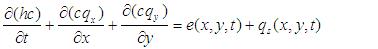(96)

where h = water depth (m); c = sediment concentration (kg m^-3); t = time (s), q_x and q_y = unit discharge in x- and y-directions, respectively (m²/s); and e(x,y,t) = sediment source/sink (kg m^-2• s^-1); q_z(x,y,t)=lateral sediment inflow to the channels (m^-2 s^-1). e(x,y,t) consists of two major sources, namely, soil detached by raindrop impact and soil detached by surface runoff (or deposition):

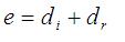(97)

where d_i=soil detachment by rainfall impact (kg m^-2• s^-1) and d_r=soil detachment by surface runoff (kg m^-2• s^-1).

10.1.2 Detachment of Overland Sediment Particles

Detachment of overland sediment particles occurs due to two processes, detachment by rainfall impact, and detachment by surface runoff.

10.1.2.1 Detachment by Rainfall Impact

Following a similar approach presented by Wicks and Bathurst [1996] and Gabet and Dunne [2003], detachment by raindrops is considered to be a function of rainfall intensity. Raindrop detachment also takes into account factors such as “cushioning” by ponded surface water, ground cover, and plant interception.

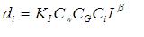(98)

where d_i = detachment capacity rate (kg m^-2 s^-1), K_I = soil erodibility factor for detachment by raindrop impact (J^-1), C_w = water depth correction factor, C_G = canopy cover factor, C_i = a cover-management factor, I = rainfall intensity (mm h^-1), and β = empirical coefficient related to rainfall intensity.

The calculation of water depth correction factor is based on the assumption that surface water depths greater than a critical depth protect the soil from raindrop impact erosion Wicks and Bathurst [1996]. The expression for the correction factor, C_w, is,

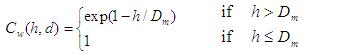(99)

where h = water depth (m), and D_m = median raindrop diameter (m). The median raindrop diameter is determined from the Laws and Parsons [1943] equation:

(100)

10.1.2.2 Surface Runoff Detachment

Surface runoff detaches soil particles by exerting a shear stress that breaks the bonds between particles. Erosion in rills is lumped and described as gross rill erosion. Within a grid cell, rill erosion and flow are assumed to be uniformly distributed. The detachment capacity rate by surface runoff has the form:

(101)

where: d_r = detachment capacity rate (kg m^-2•s^-1), a and b are empirical coefficients, τ = the flow shear stress (Pa), τ_cr is the critical shear stress, G is the sediment load (kg m^-2 s^-1), and T_c is the sediment transport capacity of surface runoff (kg m^-2 s^-1). In the WEPP model, b is assumed equal to 1.0. Equation 101 provides an upper limit on the rate at which sediment that can be taken up by flowing water.

10.1.3 Sediment transport capacity of surface runoff

Transport of sediments on the overland flow plane is constrained by the ability of the water to carry sediments. Many researchers have investigated the process and have identified multiple equations that can be used to calculate this carrying capacity of the overland flow. Several of these have been implemented in GSSHA.

10.1.3.1 Kilinc Richardson Equation

Kilinc and Richardson studied the mechanics of overland soil erosion at Colorado State University Engineering Research Center in a flume 1.2 m deep, 1.5 m wide, and 4.9 m in length. Their investigation resulted in a sediment transport equation of uniform flow sheet and rill erosion on bare sandy soil. The original one-dimensional Kilinc-Richardson (1973) equation is:

(102)

where: the factor 25,500 is an empirical constant, is the sediment unit discharge (ton m^-1 s^-1) and q and S_o have previously defined. The form of Equation 102 is consistent with many sediment transport predictors, as reviewed by Julien and Simons (1985).

Julien (1995) modified the original Kilinc-Richardson equation to expand the applicability of the equation to non-uniform flow with consideration of soil and land-use specific factors:

(103)

where: K = soil erodibility factor, with values ranging from 0 to 1, C = soil cropping factor (0-1), and P = conservation factor (0-1).

The K, C and P factors are empirical coefficients with the same conceptual meaning as those used in the Universal Soil Loss Equation (Renard et al., 1991). The factor 0.15 in the denominator represents the maximum erosivity of the sand used in the original flume experiments. Equation 103 is applied within each model grid cell in two dimensions, which allows separate calculations of the potential sediment transport rate in the x- and y-directions:

(104)

(105)

with S_ƒx and S_ƒy defined using Equation 2, and p and q calculated using Equations 6 and 7, respectively.

The numerical approach in the current version of GSSHA is to apply the modified Kilinc and Richardson equations 104 and 105 to determine potential transport of sediment within each grid cell. The methodology is explained in detail in Johnson (1997) and Johnson et al. (2000). The potential sediment discharge in each of the two flow directions in each grid cell is calculated using the following two equations:

(106)

and,

(107)

In the current version of GSSHA, the three erosioin parameters K, C, and P, have been replaced with a single erosion parameter K, which represents the three original components, without the need to specify three different parameters for each grid cell. Reducing the number of parameters greatly facilitates calibration. The form of the equation used in GSSHA is currently:

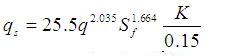(108)

where q_s is the sediment unit discharge (kg m^-1 s^-1), q is the unit discharge (m³ s^-1), S_f is the friction slope (-), and K is a combined factor(0-1) that consists of the combined influence of soil erodibility, vegetation, and land-use.

10.1.3.2 Engelund-Hansen Equation

The Engelund-Hansen [1967] relation is used to calculate sediment transport for each sediment size class and the resulting total transport is calculated by multiplying the proportion of the size in the parent material by the calculated rate.

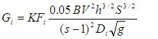(109)

where G_i is the volumetric sediment transport rate of i^th size fraction (m³ s^-1), K is the calibration coefficient (=1 for standard equation) (-), F_i is the proportion of i^-th faction in the parent material or deposited layer (-), B is the width of flow (m), V is the mean water velocity (m s^-1), h is the flow depth (m), S is the water surface slope (-), s is the specific gravity of i^th fraction (-), and g is the gravitational acceleration (m s^-2), is the sediment density (kg m^-3), is the water density (kg m^-3), D_i is the mean size of i^-th fraction (m). The factor 0.05 in the equation was developed from empirical data.

The suggested applicability of the Engelund-Hansen equation is for, where "D_N" is the grain size for which N% of sediment is finer by weight, and for sand-size sediments coarser than 0.15 mm.

10.1.3.3 Stream Power Approach

Several stream power methods [Everaert 1991] can also be chosen to calculate the transport capacity of surface runoff. The general expression has the form:

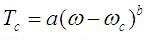(110)

where a is the transport coefficient, b is an exponent, ω = steam power; ω_c=a critical stream power. Prior to version 5.7 these values were specified by the user. For versions 5.7 and beyond the exponents are assigned based on literature values [Everaert 1991]. These there parameters are no longer input in the cmt input table file.

10.1.3.4 Median size diameter, D₅₀ , Approach

In the versions 5.7s and beyond, the Stream Power Approach defined in 10.1.3.3, are replaced by laboratory physical model imperical equations derived by Everaert [1991] which are based on the sediment particle median size diameter, D50. The replacement is done to reduce the number of calibration parameters, a, b and critical values defined in sec. 10.1.3.3.

The followings are the list of methods and their respective equations:

a) Effective stream power method:

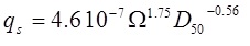- (a1)

where,

- (a2)

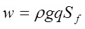- (a3)

and <math>q_s</math> = sediment unit discharge (kg/ m/ sec)

<math>D50</math> = Grain size parameter (um)

<math>\Omega</math> = effective stream power

<math>\omega</math> = stream power (N/m/s)

<math>R</math> = flow depth (m)

<math>q</math> = unit discharge (m²/s)

<math>S_f</math> = friction slope (m/m)

<math>\rho</math> = density of water at 20 C (kg/m³)

<math>g</math> = gravitational acceleration

This method is implemented if 4 is used for the project card SOIL_EROSION.

b) unit stream power method:

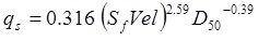- (b)

where, <math>Vel</math> = velocity (m/s)

<math>S_f</math> = friction slope (m/m)

<math>q_s</math> = sediment unit discharge (kg/ m/ sec)

<math>D_{50}</math> = Grain size parameter (um)

This method is implemented if 3 is used for the project card SOIL_EROSION.

c) slope and unit discharge method:

if(d50<33.0)

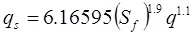- (c1)

else if(d50>=33.0 && d50<61.0)

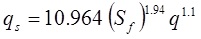- (c2)

else if(d50>=61.0 && d50<122.0)

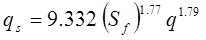- (c3)

else if(d50>=122.0 && d50<190.0)

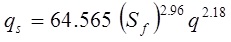- (c4)

If(d50>190.0)

- (c5)

This method is implemented if 5 is used for the project card SOIL_EROSION.

d) Transport capacity by shear velocity method:

- (d1)

u = shear velocity (m/s)

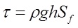- (d2)

Τ = shear stress (N/m2)

if(d50<33) and if(u>1.4)

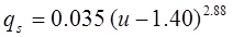- (d3)

if(d50>=33.0 && d50<61.0) and if(u>1.4)

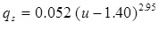- (d4)

if(d50>=61.0 && d50<122.0) and if(u>1.45)

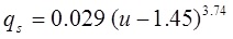- (d5)

if(d50>=122.0 && d50<190.0) and if(shear_vel>1.55)

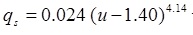- (d6)

if(shear_vel>1.8)

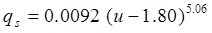- (d7)

In the above equations, D₅₀ and all other physically based hydrological, topographical and geomorphological parameters are defined by GSSHA model and need not be calibrated. As these methods are solely based on the experimental flume scale of 5 x 30 cm and 12 x 100 cm, the applicability of these lab model scale based imperical relations has been tested on catchment scale and a product of ‘constant factor’ and ‘adjustment factor’ is applied as a multiplier to each equation (a – d) in this section. Adjustment factor is a parameter for calibrating the individual equations. Constant factor is used to confine the bound of adjuistment factor between 0 and 1 while calibrating. Constant factor for each method is hard coded. We are currently assessing these methods. All of them may not appear in the next release version.

10.1.4 Deposition rate

When the sediment transport capacity is insufficient to transport the sediment in suspension within a grid cell, sediment is deposited. Sediment deposition in each grid cell is calculated for each size fraction using a trap efficiency relation [Johnson et al., 2000]:

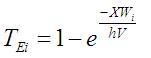(111)

where: T_Ei is the trap efficiency for the i^th size fraction, X is the width of the grid cell (m), W_i is the fall velocity of the i^th size fraction (m s^-1), h is the overland flow depth (m), and V is the overland flow velocity (m s^-1). The trap efficiency is a number between 0 and 1, which is assumed equal to the fraction of suspended sediment in each size fraction that is deposited in the grid cell. The use of trap efficiency forces larger particles to deposit before smaller particles.

10.2 Channel Sediment Transport Formulation

The present version of GSSHA employs the unit stream power method of Yang’s (1973) for routing sand-size total-load in stream channels. Unit stream power is defined as the product of the average flow velocity, U, and the channel slope S_o. The rate of work done per unit weight of water in transporting sediment is assumed directly related to the rate of work available per unit weight of water. Thus, the total sediment concentration or total bed-material load must be directly related to the unit stream power. The following relation gives the basic concept of Yang’s (1973) method:

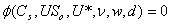(112)

where: C_s is the total concentration of sand-size sediment particles in motion, US_o is unit stream power (L/T), U_* is the shear velocity (L/T), ν = kinematic viscosity of the sediment-water mixture (L/T²), w = fall velocity of the sediment (L/T), d = particle diameter (L). With some mathematical and statistical manipulations with Buckingham’s π theorem, Yang (1973) derived an energy-based equation to estimate the total sand-size sediment concentration in the channel.

Only particles sizes larger than a user specified value for sand are transported in this manner. Smaller particles are assumed to be suspended, and not bedload, and are transported with the advection dispersion equation. The bed is assumed to be mobile, and the banks fixed. The bed can agrade or degrade to a user-specified maximum allowable depth(Figure 14).

Either trapezoidal or natural cross sections can be used. Trapezoidal channels degrade vertically into the crosshatched area in the Figure 14. Degradation continues and bed load is transported at the rate calculated with the Yang (1973) method until the maximum degradation is reached. During degradation the initial bed width is maintained and degradation is uniform across the width of the bed. If the channel aggrades, the trapezoidal cross-section is filled. If a channel link has aggraded, and then degrades, the degradation will occur uniformly over the bottom of the trapezoid until the original bed elevation is restored. Further degradation occurs vertically downward from the initial trapezoid bottom-width. If a channel, degraded below the original bed elevation begins to aggrade, sediment will accumulate uniformly in the rectangular degraded area below the original bed elevation. Once the bed aggrades beyond the original bed elevation, the entire width of the trapezoid is filled. Natural channels follow a similar pattern of agradation and degradation. The change in channel bed elevations is tracked during the simulation of the model and the final computed bed elevations are output in a file called "new_bed_elevations.txt". These new computed bed elevations are not used in the computations during the simulation unless you specify the "ADJUST_CHANNEL_BED", in which case the bed will be dynamically adjusted during the simulation, affecting all channel computations as the simulation proceeds.

In the channels size particles smaller than the user specified value of sand are assumed to be in suspension, and are transported as wash load. This treatment implies that the flow is turbulent, and the travel time to the outlet of the catchment is short compared to the settling time, such that particles do not settle in the channel network. This assumption, combined with no bank erosion, results in the channels being neither a source nor sink of fines. Routing of suspended fines is a natural extension of the explicit diffusive-wave channel routing method. Suspended fine sediments are routed as concentrations. The concentration changes as a function of gradients in both concentration and velocity.

Figure 14 – Channel bed erosion

10.3 Applicability of the Sediment Routing Methods

Ogden and Heileg (2001) performed a detailed study on the performance of the methods used in the CASC2D version 1.18 model and early versions of the GSSHA model and model and made several reccomendations to improve the formulation. Many of these formulation enhancements have included in the current version of GSSHA, v4 and higher. Additional features include the ability to specify the number, size, and specific gravity of particles, sediment detachment due to rainfall impact, refinement of the Kilinc Richardson model, and the addition of several other methods of computing transport capacity. This model has been tested against historical data sets and demonstrates improved capability over earlier versions of the model. Of note is that all sediment transport capacity equations in GSSHA contain some type of "erodibility" factor that varies betweend zero and unity. These factors are typically assigned according to land use and include the effect of many processes and contributing factors. Proper assignment of the erodibility relies on calibrating the factors with observed data. Calibrated model parameters should also be verified with independent observed data not used in the calibration effort.

10.4 Simulations with Soil Erosion

10.4.1 General

A detailed report on the soil erosion methods, estimated parameter values, and testing is available here Sediment Tech Note. Soil erosion simulations are specified with the SOIL_EROSION project card. The SOIL_EROSION card is also used to select the transport equation to be used, with an integer value of 1-6. The six transport capacity options currently are:

1 - Engelund-Hansen
2 - Kilinc Richardson
3 - Unit stream power - replaces generalized stream method formulation, new for version 5.7 and beyond
4 - Effective stream power, new for v5.7
5 - Slope and unit discharge, new for v5.7
6 - Shear stress, new for v5.7

It should be noted that methods 3,4,5, and 6 replace a generalized "stream power" method, no longer in the model. The parameters used in the generalized "stream power" method are no longer input for versions 5.7 and beyond. The following information is annotated for this change in the model.

Soil and erosion properties are assigned with the use of the Mapping Table, Chapter 11. For GSSHA versions 5.7 and up, the first three variables are not used and should not be included in the table. The eight variables are input in the following order:

 
Transport Capacity Coefficient - no longer used
Transport Capacity Exponent - no longer used
Transport Capacity Critical Value - no longer used
Rain Splash Detachment Erosion Coefficient
Overland Detachment Coefficint
Overland Detachment Exponent
Overland Detachment Critical Value
Overland Transport Capacity Erosion Coefficient

Additional optional inputs and outputs are also available. These are described in detail in Section 3.10. If channel routing is not specified in the project file only overland soil erosion calculations are performed. Sediment transport can be simulated in either event or long-term simulation mode.

There are three general categories of parameters to enter into your mapping tables when running a sediment transport simulation. These categories of parameters are explained as follows:

10.4.1.1 Overland Sediment Particle Detachment Parameters

In the formulation used in GSSHA, overland sediment particle detachment is caused in two ways: by rainfall impact detachment and by surface runoff detachment. The following input parameters are used to control how much sediment is detached by these two methods:

Rainfall Impact Detachment

Rain splash detachment coefficient (SPLASH_K)

Surface Runoff (Rill) Detachment

Overland detachment coeff (DETACH_ERODE)

Overland detachment exponent (DETACH_EXP)

Overland detachment critical shear (DETACH_CRIT)

10.4.1.2 Overland Sediment Transport Capacity Parameters

GSSHA has several equations that can be used to simulate sediment transport capacity. You can select the appropriate equation for your model based on the information in this manual and in this Sediment Technical Note. You must define and calibrate correct input parameters based on the equation you select with the SOIL_EROSION project card. The following input parameters are used to control the sediment transport equations in each of the six methods:

1 - Engelund-Hansen and 2 - Kilinc Richardson

Overland Transport Capacity Erosion Coefficient (SED_K)

3 - Unit stream power, 4 - Effective stream power, 5 - Slope and unit discharge, and 6 - Shear stress

For the current formulation of these methods, there are no adjustable parameters. Parameters previously assigned by the user, see list of parameters above, are assigned to literature values for the various methods.

10.4.1.3 Sediment Fractions

For each mapping table index, a fraction between 0.0 and 1.0 must be defined for each type of sediment defined in the simulation. The total of these sediment fractions should equal 1.0 so all sediments are included in the particle detachment and sediment transport equations.

10.4.1.4 Overview

Methods for obtaining initial values for the sediment particle detachment parameters and the sediment transport parameters are described in the following sections of this document.

10.4.2 Assignment of Overland Sediment Particle Detachment Parameter Values

The rainfall impact detachment and surface runoff detachment parameters must be initialized to correct values to get reasonable results for the detachment of sediment from the soil surface. For rainfall impact detachment, a rain splash coefficient (SPLASH_K) must be defined. For surface runoff detachment, two parameters--a runoff detachment coefficient (DETACH_ERODE) and a runoff detachment index (DETACH_CRIT) must be defined.

10.4.2.4 Rainfall Impact Detachment Parameter Values

The rain splash coefficient (SPLASH_K) entered in GSSHA is the multiplication of three factors used in Equation 98, which determines rainfall impact detachment. SPLASH_K = (K_I)(C_G)(C_i)

10.4.2.4.1 K_I

K_I is the soil erodibility factor for detachment by raindrop impact. The units for this factor are J^-1 (1/Joules) and the value is approximated using the table 2 from Wicks and Bathurst [1996], shown below:

Soil Texture	Raindrop Erodibility Factor KI, J-1 Meyer and Harmon (1984)	Raindrop Erodibility Factor KI, J-1 Morgan (1985)	Raindrop Erodibility Factor KI, J-1 Bradford et al. (1987 a,b)	Raindrop Erodibility Factor KI, J-1 Verhaegen (1987)
Clay	19.0		73.5
Silty Clay	18.2
Silty Clay Loam	16.2		22.2
Silt	29.8
Silt loam	39.8		25.7	24.7
Loam	28.2	30.0	37.6	23.4
Sandy Loam	32.0		34.4	30.0
Sand			62.4

10.4.2.4.2 C_G

C_G is the ground cover factor and is a value between 0.0 and 1.0. This factor = 1.0 - Fraction of ground covered by ground cover. This factor is unitless and can be obtained from a land use map, a ground cover map, or an aerial photograph.

10.4.2.4.3 C_i

C_i is the cover-management factor and is a value between 0.0 and 1.0. This factor = 1.0 - Fraction of ground covered by canopy cover. This factor is unitless and can be obtained from a land use or a canopy/vegetation cover map or a recent aerial photo of the area being modeled.

10.4.2.5 Surface Runoff Detachment Parameter Values

GSSHA uses three surface runoff detachment parameter values that must be entered in your GSSHA model. The runoff detachment coefficient (DETACH_ERODE, a), the runoff detachment index (DETACH_INDEX, b), and the runoff detachment critical shear (DETACH_CRIT, τ_cr) are used in Equation 101, which determines surface runoff detachment.

10.4.2.5.1 Runoff Detachment Coefficient, a

According to the Water Erosion Prediction Project (WEPP) model documentation, a value of 0.004 for rangeland and a value of 0.05 for cropland should be used for the runoff detachment coefficient.

10.4.2.5.2 Runoff Detachment Index, b

According to the Water Erosion Prediction Project (WEPP) model documentation, a value of 1.0 should be used for the runoff detachment index.

10.4.2.5.3 Runoff Detachment Critical Shear, τ_cr

τ_cr is the runoff detachment critical shear. The units for this factor are Pascals and research is still being conducted on how to obtain this value. We recommend using the default value of 3.5 Pa for this value.

10.4.3 Assignment of Overland Sediment Transport Parameter Values

The Kilinc Richardson and Engelund Hansen transport capacity formulations in GSSHA (Equations 108 and 109) require an erodibility coefficient (SED_K, or K) that varies between zero and unity. As originally formulated for CASC2D, the erodibility factor for the Kilinc Richardson equation contained three factors K, C, and P, that were combined in the equation to describe the overall erodibility of the soil, including the effects of soil texture, vegetation coverage, and management practices. Lower values indicate less erodibility. Although only one factor is currently used in GSSHA, this single factor represents the combined effects of the three original factors contained in the original Kilinc Richardson formulation, as well as other factors. The combined erodibility can thus be assigned based on three original factors as described.

Downer et al (2010) states that the Engelund-Hansen equation is applicable for soils in which <math>\sqrt{D_{75}/D_{25}} < 1.6</math> and for sand-size sediments coarser than 0.15 mm.

The other stream power transport formulations require three parameters that are described in Equation 110 and below.

Downer et al (2010) states that a comparison of the three sediment transport relations in Equations 108, 109, and 110 (Kilinc Richardson, Engelund Hansen, and Stream Power) was performed by running the GSSHA model with each equation. Surprisingly, the result of this comparison showed that for sediments with S=2.65, there is very little difference between them. Therefore, the user is advised to use the Kilinc-Richardson method because it has the smallest number of parameters. However, for simulations involving sediments with specific gravities different from 2.65, the use of the Engelund-Hansen equation is required.

10.4.3.1 Erodibility Coefficient, K

The general erodibility, K, is based on the composition of the soil in each cell. This erodibility can be reduced by vegetative or other coverage with the C factor, and can be further reduced, or increased, by the management practice factor, P. The erodibility coefficient, SED_K = (K)(C)(P).

Soil erosion parameters and soil erosion factors may be estimated from land use, vegetation, and soil texture indices. These values are entered with in the Mapping Table File.

10.4.3.1.1 Soil Erodibility (K)

Soil erodibility describes the susceptibility of the soil to detachment and transport by rainfall impact and overland flow. Soil erodibility is generally a function of soil texture, soil structure, organic content, and permeability. In general, larger particles are harder to erode, as are undisturbed soils. Organic soils are less susceptible to erosion, and have lower K values. The values in Table 17, from Wanielista (1978), are for undisturbed, inorganic soils.

Soil Texture	Erodibility Factor K
Sand	0.05
Loamy sand	0.12
Sandy loam	0.27
Loam	0.38
Silt loam	0.48
Sandy clay loam	0.27
Silt	0.60
Clay loam	0.28
Silty clay loam	0.37

Table 17 – Soil erodibility factor (K) of the modified Kilinc Richardson Equation, Wanielista (1978)

10.4.3.1.2 Cropping Management Factor (C)

The cropping management factor (C) describes the effect of land coverage on reducing the erodibility of bare soils. In general, covered lands are less susceptible to erosion, and have lower C values. With no cover on the soil, the full erodibility (K) can be achieved, and C=1.0. Table 18 lists values for general land coverage types.

Cover	Cropping Factor C
None (fallow)	1.00
Native vegetation	0.01
Crops	0.08
Pasture	0.01
Forest	0.005
Urban	0.01
Other	1.0

Table 18 – Cropping management factors (C), Wanielista (1978) and Goldman et al. (1986)

10.4.3.1.3 Conservation Practice Factor (P)

The conservation practice factor reflects efforts specifically intended to reduce erodibility of the soil. This factor is generally associated with practices used by farmers to conserve the soil, such as no-till and contour farming. This factor may also be important for certain types of construction practices, such as coverage with geotextiles, which tend to reduce erodibility. Other construction practices, such as smoothing and compacting the soil, actually increase erodibility and can result in the value of P being greater than 1.0. Table 19 lists recommended values of P for general land use.

General land use	Control Practice Factor P
Crop	0.5
Pasture	1.0
Forest	1.0
Urban	1.0
Other	1.3

Table 19 – General landuse erosion control factors (P), Wanielista (1978)

10.4.3.2 Stream Power Coefficients, a, b, and ω_c - no longer assigned

The stream power transport formulations require three parameters, a, b, and ω_c, that are described in Equation 110. In this equation, a is a transport coefficient, b is an exponent, and ω_c is a critical stream power. In GSSHA, these are called, respectively, the transport coefficient (TC_COEFF), the transport index (TC_INDEX), and the critical transport capacity (TC_CRIT). In GSSHA version 5.7 and beyond, these parameters no longer assigned by the user. The values are set internally to literature values. These paramters should not be included in the sediment mapping table when using GSSHA versions 5.7 and beyond.

10.4.3.2.1 Transport Coefficient, a - no longer assigned

The Transport Coefficient (TC_COEFF) is used in the stream power equation. No advice is available for determining this parameter from watershed data, so it is recommended that you use Kilinc-Richardson equation (Equation 108) and use the default value of 0.285 for this coefficient.

10.4.3.2.2 Transport Index, b - no longer assigned

The Transport Index (TC_INDEX) is used in the stream power equation. No advice is available for determining this parameter from watershed data, so it is recommended that you use Kilinc-Richardson equation (Equation 108) and use the default value of 1.3 for this coefficient.

10.4.3.2.3 Critical Transport Capacity, ω_c - no longer assigned

The Critical Transport Capacity (TC_CRIT) is used in the stream power equation. No advice is available for determining this parameter from watershed data, so it is recommended that you use Kilinc-Richardson equation (Equation 108) and use the default value of 0.0002 for this coefficient.

10.4.4 Adjusting Overland Elevations during Sediment Simulations=

Unless specified with the ADJUST_ELEV card, changes in elevation due to erosion and deposition are not tracked during the simulation. If the user wishes to include the ongoing effect of erosion and deposition on hydrologic processes during the simulation, the ADJUST_ELEV project card is used to specify this option and to specify the name of a file that will contain the final elevations (in a GRASS ASCII map) at the end of the simulation. The volumetric change in each cell, positive for deposition and negative for erosion can be output using the NET_SED_VOLUME card regardless of whether the ADJUST_ELEV card is used or not so that the user need not include the ADJUST_ELEV card just to get information about the net gain/loss of sediment over the duration of the simulation. The primary purpose of the ADJUST_ELEV card is to include the effects of erosion and deposition on the elevations used during the simulation.

10.4.5 Channel Routing of Sediments

If explicit channel routing is specified in the project file with the CHAN_EXPLIC or DIFFUSIVE_WAVE project cards along with the SOIL_EROSION project card, sediment routing in channels will also be performed. In the CHAN_INPUT file, the user specifies the initial cross-section of each channel link. For each erodible link the maximum depth of erosion is specified with the MAX_EROSION card. Proper construction of a channel input file is given in Section 5 of this manual.

10.4.6 Output

When simulating sediment routing the volumetric flux of sediment at the outlet (cms) is output with the project card OUTLET_SED_FLUX followed with the name of the file for the output. This is a REQUIRED card. The outlet sediment flux will be output at the channel outlet, if channel routing is specified, or at the specified overland flow outlet cell. The format of the outlet sediment flux is a time stamp followed by a column of flux (cms) for each sediment particle specified in the mapping table file. Wash load particles are listed first, in the order specified in the mapping table file, followed by the sand and larger size particles, also in the order specified in the mapping table file. In addition to the specified sand size particles there is one additional column for sand or larger sizes that represents the bed load originally in the channel, so that even if no sand size particles are specified in the mapping table file, the user will still see one column representing bed load for the initial channel sediments. If channel routing is being conducted, then the same information can be output at interior link/node locations using the IN_SED_LOC card, to specify the desired sedograph link node pairs, and the OUT_SED_LOC card which specifies the name of the file that will contain sedographs at the desired locations. The information in the OUT_SED_LOC file will be same as in the OUTLET_SED_FLUX file, except there will be a series of data for each chosen output link/node pair. Data from the link/node pairs in the OUT_SED_LOC file will be listed in the order they were specified in the IN_SED_LOC file. The format of the IN_SED_LOC file is exactly the same as the format for the IN_HYD_LOCATION file, and if the same points are desired for sediment flux as flow, then the same file can be used for both. Additionally, the concentration (mg/L) of total suspended sediments (TSS) at the outlet can be output with the OUTLET_SED_TSS card which is used to specify the file for the outlet TSS information. TSS at interior points can be specfied using the OUT_TSS_LOC card. The link node pairs for the OUT_TSS_LOC file are specified in the file named by the IN_SED_LOC card. Additional information about the output available for sediment processes can be found in Section 3.13.3 of the User's Manual.

Maps of the maximum sediment flux (cms) and the volumetric change (m3) can be output using the MAX_SED_FLUX and NET_SED_VOLUME cards, respectively. Additional information about the output available for sediment processes can be found in Section 3.13.3 of the User's Manual.

---

---

 

11 - Constituent Transport and Fate

GSSHA User's Manual

11.1 Simulating Reactive Constituents in GSSHA

Reactive constituent transport can be simulated on the overland flow plane, the channels including reservoirs, and in the soil. Most commonly, constituents will be simulated in both the overland flow plane and in the channels. It is possible to simulate constituents in the channels alone, if a point source of contaminants is introduced to the channel. Simulation of constituents in the soil column requires that constituents are simulated on the overland flow plane as well. A description of the methods is described in detail in Downer 2009 WQ TN and Downer and Byrd (2007): TMDL TN

11.1.1 - Simulation of Constituents on the Overland Flow Plane

Constituents are simulated on the overland flow plane by including the OV_CON_TRANS card in the project file. The only way to specify parameter values for overland constituent transport is in the MAPPING_TABLE file. Details of the required MAPPING_TABLE inputs are specified in Section 12. The inputs required depend on the type of constituents selected for simulation. Constituents can be simple (first order) or NSM (full nutrient cycle).

Two types of reactive constituent transport are available in GSSHA. Constituents can be simulated as simple first order reactants with specified uptake rates from the soil and specified decay rates. The nutrient cycle can also be simulated with the Nutrient Simulation Model (NSM) (Johnson and Gerald, 2008). In either case, the overall simulation methods within the GSSHA model are the same. Only the rates of mass absorption and decay are different. It is therefore possible to simulate nutrients as simple constituents, as well as simulating them with the full nutrient cycle. It is up to the user to determine the appropriate level of chemical kinetics for the problem to be solved. More on both of these options is provided in subsequent sections.

In addition to reactions and transformations, contaminants on the overland flow plane are gained and lost due to:

1. Addition by rainfall
2. Uptake from the soil surface
3. Exchange with soil
4. Infiltration
5. Exchange with channels
6. Exchange with groundwater
7. Addition by point sources
8. Exchange with reservoirs

More detail on the methods used in GSSHA are provided in Downer and Byrd (2007): TMDL TN

11.1.1.1 - Addition by Rainfall

The concentration in precipitation (g m^-3) of each constituent being simulated is constant throughout the simulation. The rainfall concentration for each contaminant is specified in the MAPPING_TABLE file. Rainfall inputs are added directly to the overland flow plane, where they may either infiltrate, or pond and produce contaminated runoff.

11.1.1.2 - Uptake from the Soil Surface

Contaminants on the overland flow plane can be considered in one of two ways. They can be considered to be laying on the soil surface, or they can be considered to be mixed in the soil column. The default is that contaminants are present on the soil surface. The amount of contaminants (Kg) is specified for each cell in the MAPPING_TABLE file. Then, the uptake coefficient (K) (m d^-1), specified for simple constituents in the MAPPING_TABLE file and calculated for NSM, is used to move the contaminants into the overland flow based on the concentration deficit (solubility of the constituent and the concentration in solution). For simple constituents these parameters are specified in the MAPPING_TABLE file. For nutrients, these calculations are performed by the NSM. The flux (F) (g s^-1) is computed as

F=KA(Cmax -C)/86400.0

Where Cmax is the maximum concentration (g m^-3) of the contaminant (solubility), C is the concentration of contaminant in the ponded surface water, and A is the area of the computational grid cell (m²). The value 86400.0 converts the reaction rate (K) into (m s^-1);

11.1.1.3 - Exchange with Soils

Optionally, contaminants distributed on the overland flow plane at the beginning of the simulation may be mixed into the soil column by including the SOIL_CONTAM card in the project file. Currently, any of the Green and Ampt models of infiltration can be used to simulate constituents in the soil column: Green and Ampt, INF_GA, the Green and Ampt with redistribution INF_REDIST (GAR) model of infiltration (Ogden and Saghafian, 1997) coupled to the two layer soil moisture model (Downer, 2007), and the multi-layered Green and Ampt model INF_LAYERED_SOIL. The Richard's equation cannot be used for soil contaminant transport. When simulating constituents in the soil column the concentration of contaminants in the soil (mg/Kg) is specified in the MAPPING_TABLE file over a specified mixing depth in the soil column. The mixing layer depth (m) is specified with the MIXING_LAYER_DEPTH card which specifies an additional layer in the soil column: resulting in two layers for INF_GA, two or three layers in INF_REDIST and three layers in INFL_LAYERED_SOIL.

Constituents in the soil partition between the soil matrix and the pore water based on the chemical properties, the soil properties, and the soil moisture. Constituent uptake into water ponded on the overland flow plane occurs due to the uptake rate (K) and the concentration difference between the soil pore water volume and the overland flow plane. As the concentration gradient may be in either direction, the flux may also be in either direction, i.e. the flux may be into the soil, acting as a sink for the overland plane. How constituents are treated in the soil column are discussed in detail below.

During simulations uptake, decay, and movement between layers will change the concentration in the surface soil layer, as described above. The concentration of materials in the surface soil layer can be held static by using the SOIL_STATIC_CONC card in the project file. This might be desirable when either the concentration in the soil is expected to held constant by addition of more constituent, such as N and P addition due to fertilizer. Furthermore, fluxes between soil layers can be halted by using the SOIL_NOFLUX card. This might be desirable to include if the material in the top layer is being flushed out at an excessive rate and reducing the surface soil layer concentration too rapidly. This option may also be desirable to use if exfiltration is occurring and an excessive amount of constituent is being added to the overland flow plane.

11.1.1.4 - Infiltration

Some or all of the water ponded on the land surface may infiltrate, removing contaminants. Water that infiltrates is assumed to contain the same concentration of dissolved contaminants as the ponded water. All G&A models of infiltration work with contaminants in the soil column.

11.1.1.5 - Exchange with Channels

In general the overland flow plane acts as the primary source of contaminants to the channel, and this is a sink. For cases where the OVERBANK card is specified in the project file, along with channel routing, the stream may overflow and add water, as well as constituents, back to the overland flow plane.

11.1.1.6 - Groundwater

The overland flow plane interacts with the groundwater in two possible ways. If the groundwater table is high enough, water may spill out onto the overland flow plane as exfiltration. If the SOIL_CONTAM option is not specified, water spilling back on the overland flow plane has the specified groundwater concentration for that cell. If the SOIL_CONTAM card is in the project file, the concentration will be calculated as part of the soil constituent transport routine, as descibed below. Constituents seeping out of the soil column into the groundwater are accounted for but do not affect the static groundwater concentration for the cell. If exfiltration is occurring, water will enter the soil column from the bottom with concentration specified for the groundwater in that cell. Water seeping onto the surface will also have this concentration. In some cases this action may lead to an excess of constituent being added to the land surface. In that case, using the SOIL_NOFLUX card will stop the addition of constituent onto the land surface from groundwater seepage.

11.1.1.7 - Point Sources

Point sources may be input into any cell in the watershed. Point sources are defined in the OV_POINT_SOURCE file. The OV_POINT_SOURCE file contains the number of points (N) and the i and j location (or link and node), discharge rate, a flag if the location is for a channel (1) or the grid (0), Q (m³ s^-1), and concentrations, C (mg L^-1), for all constituents of each point source as shown below. In the example below, there are N point sources and M constituents.

[# Point sources (N)] [cell i/link point source 1] [cell j/node point source 1] [is_channel] [Q1] [C1,1] [C1,2] [C1,3] ... [C1,M] [cell i/link point source 2] [cell j/node point source 2] [is_channel] [Q2] [C2,1] [C2,2] [C2,3] ... [C2,M] ... [cell i/link point source N] [cell j/node point source N] [is_channel] [Q3] [CN,1] [CN,2] [CN,3] ... [CN,M]

Values in the table are separated by spaces.

11.1.1.8 - Exchange with Reservoirs

Reservoirs in the channel network are also present within the overland flow plane (Downer et al., 2008). Water and constituents may be lost to a reservoir by either flowing into the reservoir, or by the reservoir rising and taking over the overland flow cell. Water and constituents may also flow from the reservoir back onto the overland flow plane. This results in a source for the overland cells adjacent to the rising reservoir.

11.1.2 - Simulation of Constituents in the Channel Network

Simulation of constituents in the channel network is specified by including the CHAN_CON_TRANS card in the project file. Typically, the source for contaminants in the channel is derived from inputs from the overland flow plane. Contaminants may also be added to the channel from groundwater exchange. As contaminants are not currently simulated in the groundwater, static values of contaminant concentration are specified for the groundwater. Contaminants may also be added to the channels as point sources. If CHAN_CON_TRANS is specified in the project file without OV_CON_TRANS transport will be computed only in the channel network. In this case, the only possible sources are point sources.

Transport of constituents within the channel network is calculated with the general 1-D advection-dispersion equation in terms of the mass of constituent (M) equal to the concentration (C) multiplied by the volume (V) with constant dispersion. The details of the equations are described in Downer and Byrd (2007). For the channels, the following sources/sinks are considered in addition to chemical reactions.

1. Exchange with overland flow
2. Exchange with reservoirs
3. Exchange with groundwater
4. Point sources

11.1.2.1 Exchange with Overland Flow

As described above for overland flow, water from the overland flow plane is deposited in the stream network in overland grid cells that contain all or part of a stream node. If the channel spills back onto the overland flow plane, this is treated as sink in the channel calculations. Water can only spill back onto the overland flow plane if the OVERBANK card is included in the project file.

11.1.2.2 Exchange with Reservoirs

As described in Downer et al. (2008) stream networks may contain reservoirs. Water and constituents are lost to the channel in two ways. Water may flow into the reservoir from one or more upstream tributaries. The reservoir may also expand, taking stream nodes or entire reaches. When this occurs, any water and constituents in the overtaken stream node is removed from the channels and added to the reservoir. Reservoirs are treated at completely mixed reactors for flow, sediments, and contaminants. Decay, exchange with sediments, and settlement of attached contaminants can occur. Discharges from reservoir outlets act as sources to the channel network.

11.1.2.3 Exchange with Groundwater

Channel losses can be simulated whether or not the saturated groundwater surface is included in the simulation. When water seeps into the channel bottom, subsequent loss of constituents occurs as well. When the water table is included in the solution, as either static or varying, exchange can be in either direction. Concentration of constituents is specified for every cell in the groundwater domain. This concentration does not vary in time throughout the simulation. If flow is from the groundwater domain to the channel, water entering the channel is assumed to have the specified groundwater concentrations of constituents. Seepage from the channel to the groundwater is assumed to have the same concentration as the water in the channel node. Additions and subtractions to the groundwater are accounted for but do not affect the specified groundwater concentrations.

11.1.2.4 Point Sources

Point sources may be input into any node in the stream network. Point sources are defined by a constant discharge rate and concentration for each point source.

Point source flows and concentration of contaminants can be input using the CHAN_CON_INPUT table which contains one line with the number of point sources (N) in the file and one line with the node and link numbers, flow, Q (m³ s^-1) , and concentration, C (mg L^-1), for each point source as shown below.

# Point sources (N)
Node #     Link #     Q1     C1 
Node #     Link #     Q2     C2
Etc.
Node #      Link #     QN-1     CN-1

Node #      Link #     QN     CN

11.1.2.4 Defining Paramter Values

Initial concentrations (g m^-3), decay coefficients (d^-1), and dispersion coefficients (m² s^-1) are needed for each node, and are input as uniform values for the entire stream network using the INIT_CHAN_CONC, CHAN_DECAY, and CHAN_DISP_COEF project cards, respectively. In-stream partition coefficients for each constituent are taken from the constituent mapping table file.

11.1.3 Soil column Transport

Simulation of contaminants in the soil column is selected by including the SOIL_CONTAM card in the project file. For simulations of transport in the soil column, infiltration must be simulated with one of the Green and Ampt infiltration models, such as the GAR infiltration model (INF_REDIST) and soil moisture must be simulated with the simple soil moisture accounting routine. The simple soil moisture accounting routine (Downer, 2008) allows the user to specify up to two soil layers for computations of soil moisture (SOIL_MOIST_DEPTH and TOP_LAYER_DEPTH). The method is similarly applied to the multi layered Green and Ampt model.

Within these layers downward soil water movement is due to gravity. If groundwater is being simulated, the groundwater may rise into the soil column, causing an upward flow of water in the soil column. Soil movement due to capillary pressure is not considered. Infiltration is a source to the top layer. Leakage from the bottom layer is considered a loss. Loss of water, but not constituents, also occurs due to ET, which is taken from both soil moisture layers.

Figure 2 shows the conceptual model of the soil column transport model. Downward fluxes (infiltration, gravity drainage, groundwater recharge) are shown on the left. Upward fluxes (exfiltration, upward groundwater flux) are shown on the right. Diffusive exchange occurs between the top soil layer and the surface water. Exchange between pore water and soil particles occurs in every layer, as does decay and transformations.

Figure – Soil column transport model

During simulations uptake, decay, and movement between layers will change the concentration in the surface soil layer as defined above. The concentration of materials in the surface soil layer can be held static by using the SOIL_STATIC_CONC card in the project file. This might be desirable when either the concentration in the soil is expected to held constant by addition of more constituent, such as N and P addition due to fertilizer. Furthermore, fluxes between soil layers can be halted by using the SOIL_NOFLUX card. This might be desirable to include if the material in the top layer is being flushed out at an excessive rate and reducing the surface soil layer concentration too rapidly. This option may also be desirable to use if exfiltration is occurring and an excessive amount of constituent is being added to the overland flow plane.

11.1.3.1 Distribution of Constituents in the Soil Column

When simulating constituents, an additional transport layer may be included in the soil transport calculations by including the MIXING_LAYER_DEPTH card in the project file. The MIXING_LAYER_DEPTH is specified in meters. Specification of this layer further divides the surface soil moisture layer. Any initial amount of constituents distributed on the overland flow plane is assumed to be mixed within the MIXING_LAYER_DEPTH. If this additional layer is not specified in the project file, the initial amount of contaminants is assumed to evenly mixed over the TOP_LAYER_DEPTH if using INF_REDIST, and there will be only two layers in the soil transport model. If using only one soil moisture layer with INF_REDIST specified with the SOIL_MOIST_DEPTH, then the initial amount of constituents is assumed to be mixed over this single layer, and transport is computed for one soil layer only. If using INF_LAYERED_SOIL the top soil layer is assumed to be the MIXING_LAYER_DEPTH unless otherwise specified with the MIXING_LAYER_DEPTH card.

Regardless of the total number of layers, the initial constituent loading specified in the MAPPING_TABLE is assumed to be mixed over the depth of the top layer. This mass of contaminants is distributed between an amount absorbed to the soil and dissolved in the pore water. The distributrition is calculated based on the chemical partition coefficient and the soil moisture as described by Johnson and Gerald (2007). For simple constituents, values of the partition coefficient are specified in the MAPPING_TABLE. A partition coefficient value is specified for each mapping table category for each contaminant.

11.1.3.2 Exchange with Surface Water

During the simulation, infiltration acts as a source to the top layer. Advection of water transfers water and constituents to lower layers. Leakage from the bottom layer is a sink for that layer. The concentration of constituent in the advected water depends on the mass of contaminant in the layer, the soil moisture, and the partition coefficient.

Exchange with water ponded on the land surface occurs due to the concentration gradient between the pore water in the top soil layer and the ponded water. The flux (F) (g s^-1) is calculated as:

F=KA(C_ponded-C_soil)/86400.0

Where: C_ponded is the concentration in the water ponded on the soil surface, C_soil is the concentration in the soil pore water, and K is the kinetic rate (m d^-1), and A is the area of the computational grid cell (m²). The value 86400.0 converts K from per day to per second. As can be seen in the equation, the direction of the flux is dependent of the relationship between the concentration of the surface water to the soil pore water volume.

11.1.3.3 Interaction with Groundwater

If the water table is being simulated, the water table may be present in any or all of the soil layers. If the water table is present in a layer, the amount of groundwater in that layer is considered in the calculation of soil moisture in the layer for the purposes of partitioning the constituent between dissolved and attached fractions.

If exfiltration occurs, the groundwater is considered to come into the bottom layer, reach equillibrium condition in that layer and then move upward to the next layer, where it reaches equilibrium before being advected upward to the next layer, and ultimately to the land surface. However, the concentration of water exfiltrating at the land surface is assumed to be at the groundwater concentration, not the surface soil layer concentration. In practice, this approach proves superior to using the calculated surface layer concentration. In cases where exfiltration is causing excessive constituent to be added to the overland flow plane, the SOIL_NO_FLUX card can be used, which will result in no fluxes of constituent between soil layers, including exfiltration.

11.1.4 Reservoir Transport

Reservoirs in the stream network are treated separately from the channel network. Each reservoir is considered as a completely mixed reactor. As described above, reservoirs interact with both the overland flow plane and the channel network. Reservoirs can also interact with the groundwater in the same manner as the channels, where the reservoir water and contaminants can seep to the groundwater, and the groundwater can supply water with static concentrations to reservoirs.

11.1.5 Groundwater Transport

GSSHA does not currently simulate fate and transport in the saturated groundwater. Whenever a water table is simulated in the GSSHA model, a concentration is specified for every grid cell in the watershed. Any flux from the groundwater to any other domain has the static constituent concentration of the groundwater cell that the flux occurs from. Fluxes to and from the groundwater do not affect the groundwater concentrations. This simplified conceptualization of groundwater may not be adequate for simulating conditions where the groundwater exchange is significant and the groundwater concentrations vary with time over the period of the simulation.

11.2 Transport Formulations

The methods used in transporting reactive constituents in GSSHA for the overland flow plane and channels are descibed in Downer and Byrd 2007.

TMDL TN

11.3 Simple Constituents

As described in Section 11.1, reactive contaminants may be treated as simple constituents. That is, all reactions are simple first order reactions with user specified kinetic rates (K). There is no limit on the number of simple constituents that can be simulated at one time.

11.3.1 Overland Flow Plane

For the overland flow plane kinetic rates and other inputs are specified in the MAPPING_TABLE_FILE. For each contaminant a single value of rainfall concentration (mg L^-1) is specified. All other input values are distributed both by constituent and location on the overland flow plane with the index map and mapping table values. The following table inputs are required.

1. Dispersion coefficient on the overland (m² s^-1)
2. Decay coefficient in the soils and the overland K (d^-1)
3. Uptake coefficient K_u (m d^-1)
4. Initial loading (Kg) or (mg Kg^-1)
5. Groundwater concentration (g m^-3)
6. Initial concentration (g m^-3)
7. Soil water distribution coefficients in the soil K_d (L Kg^-1)
8. Solubility C_max (g m^-3)

See Section 13 for details on the MAPPING_TABLE inputs.

Three types of reactions can take place on the overland flow plane:

1. uptake from land surface,
2. uptake from soil,
3. decay.

1) The uptake coefficient controls movement of contaminants into the overland flow based on the concentration deficit (solubility of the constituent and the concentration in solution). The mass flux (F) (g s^-1) is computed as:

F=K_u A(C_max -C)/86400.0

Where C is the concentration of contaminant in the ponded surface water, and A is the area of the computational grid cell (m²). The value 86400.0 converts the reaction rate into (m s^-1).

2) If SOIL_CONTAM is included in the project file K_u is the transfer rate between the soil pore water and the water ponded on the land surface. In this case the mass flux (F) (g s^-1) is calculated as:

F=K_u A(C_ponded-C_soil)/86400.0

Where: C_ponded is the concentration in the water ponded on the soil surface, C_soil is the concentration in the soil pore water. The value 86400.0 changes the reaction rate from per day to per second. As can be seen in the equation, the direction of the flux is dependent on the relationship between the concentration of the surface water to the soil pore water volume.

While the uptake coefficient is generally considered a calibration coefficient, for contaminants in the soil column the uptake coefficient can be estimated from Thibodeaux, Environmental Chemodynamics 2nd Ed., Wiley, New York, 1996, pp. 276-277 using the relation:

K_u = D n^4/3/(0.5 d_ml)

where D is the diffusion coefficient of the chemical in water (m² s^-d), n is the porosity, d_ml is the mixing layer depth (m).

Thibodeaux list a diffusion coefficient for nitrates of 0.000164 m² d^-1. For a typical soil with porosity of 0.4 and a mixing layer depth of 0.1 m, the uptake coefficient for nitrate would be 0.001 m d^-1. Lerman, Geophysical Processes, Wiley, New York, 1979, pp. 73-121, lists diffusion coefficients for common ions. It should be noted that effective values for of uptake coefficients for nitrate used in previous modeling efforts, for example Pradhan et al. (2014), have been much lower, on the order of 10^-5 m d^-1.

Pradhan, N. R., C. W. Downer, and B. E. Johnson, 2014. A Physics Based Hydrologic Modeling Approach to Simulate Non-point Source Pollution for the Purposes of Calculating TMDLs and Designing Abatement Measures, Chapter 9 in Practical Aspects of Computational Chemistry-III, DOI 10.1007/978-1-4899-7445-7_1, J. Leszczynski and M. K. Shukla, eds. Springer Science+Business Media, New York.

3) Contaminants dissolved in surface water decay at the rate:

F=KCV/86400.0

where V is the volume (m³), A times the depth.

11.3.2 Channels

For channels, the only reaction is decay, calculated as above. The decay coefficient can be set as a uniform value for every stream node by specifying the value (d^-1) with the CHAN_DECAY card. In addition to setting the rate, the dispersion coefficient (m²s^-1) can be defined with the CHAN_DISP_COEF card. Inital values (g m^-3) can be specified with the INIT_CHAN_CONC card. The default value for each of these is zero. The partition coefficient is the same as for the overland.

11.3.3 Soil Column

When transport in the soil is specified with the SOIL_CONTAM card, exchange between the top soil layer and the surface water occurs, as well as decay in the soil pore water. The reactions are the same as described above for overland flow. The soil water distribution coefficient controls the pore water concentration. The fraction of the total that is dissolved is:

where theta is the soil moisture (fraction) and rho_s is the dry soil density (Kg m^-3). So that the concentration dissolved is:

C_d=f_dM/V

where: M is the total mass in the layer (g) and V is the volume of the pore water in the soil layer (m³).

The same reaction rates specified in the MAPPING_TABLE_FILE are used for both the soils and the overland flow.

During simulations uptake, decay, and movement between layers will change the concentration in the surface soil layer, which can be specified as the MIXING_LAYER_DEPTH, or if using INF_REDIST is the top layer depth, either TOP_LAYER_DEPTH or SOIL_MOIST_DEPTH depending on whether one or two soil infiltration layers are specified, or if using INF_LAYERED_SOIL the MIXING_LAYER_DEPTH or the top infiltration layer in the soil profile. In any case the concentration of materials in the surface soil layer can be held static by using the SOIL_STATIC_CONC card in the project file. This might be desirable when either the concentration in the soil is expected to held constant by addition of more constituent, such as N and P addition due to fertilizer. Furthermore, fluxes between soil layers can be halted by using the SOIL_NOFLUX card. This might be desirable to include if the material in the top layer is being flushed out at an excessive rate and reducing the surface soil layer concentration too rapidly. This option may also be desirable to use if exfiltration is occurring and an excessive amount of constituent is being added to the overland flow plane.

11.4 Point and Non-point sources

Point and Non-point Sources

In addition to the point sources described in the transport section, there is method for specifying time varying point and non-point sources. These point and non-point sources are set up as discrete entries in the point/non-point source file. All of the point and non-point sources are specified as having time varying flows and either 1) a time varying mass input or 2) time varying concentration inputs. To create a constant flow, mass, or concentration, simply put a single time value in the time series. All of these time series will need to be set up in a time series file or files and those files specified in the project file. For more information, see the section of the manual on time series formats.

11.4.1 Project Card

The project card for the point/non-point source file is:

SOURCE_FILE	"filename.src"

11.4.2 File Header

The first line of the file should be a header line identifying the file:

CONSTITUENT_SOURCEFILE

11.4.3 File Organization

The point/non-point source file first sets up specific names for each the point and non-point source spatial distributions. There should be at least one link/node or cell in the distribution file, and there may be more than one (for point sources). For overland point sources, use the SOURCECELLS card and use SOURCENODES for the stream sources. For overland non-point sources, use the SOURCEGRID card.

SOURCECELLS  "source_name"  "distribution_file_name.ext"
SOURCENODES  "source_name"  "distribution_file_name.ext"
SOURCEGRID   "source_name"  "distribution_index_map.ext"

The distribution file is described below.

After the SOURCECELLS and SOURCENODES cards come the point source and non-point source records

11.4.4 Point Sources

Point sources are for inputs that are part of some flow into the domain. These would be outfall points or similar things. The flow specified in the point sources is added to the model as a source into either the overland domain or the stream domain, depending on the type of source chosen (what source type "source_name" is,) and the mass/concentration added to the mass/concentrations of the constituent in the location(s) specified by the "source_name."

POINTSOURCE  "source_name"
FLOW "ts_name"
[constituent_card] [inputs…] 
[constituent_card] [inputs…] 
[constituent_card] [inputs…] 
… 
END_POINTSOURCE

Where the constituent cards and their inputs are from the following

NO2_MASS "mass time series name"
NO2_CONC "concentration time series name"
NO3_MASS "mass time series name"
NO3_CONC "concentration time series name"
NH4_MASS "mass time series name"
NH4_CONC "concentration time series name"
ON_MASS "mass time series name"
ON_CONC "concentration time series name"
OP_MASS "mass time series name"
OP_CONC "concentration time series name"
DP_MASS "mass time series name"
DP_CONC "concentration time series name"
ALG_MASS "mass time series name"
ALG_CONC "concentration time series name"
CBOD_MASS "mass time series name"
CBOD_CONC "concentration time series name"
DO_MASS "mass time series name"
DO_CONC "concentration time series name"
GENERIC_MASS [constituent #] "mass time series name"
GENERIC_CONC [constituent #] "concentration time series name"

Masses are specified in units of kg, while concentrations are specified in units of mg/l.

11.4.5 Non-point Sources

The non-point sources are for loadings that are not dependant upon flow but rather are simply placed across the land surface. Thus, All non-point source loadings are masses, not concentrations. There are two types, instantaneous and continuous. For the continuous loadings, the units are in kg/day/m2. For the instantaneous loadings, the entries in the time series should be just the times of application, and the values should be in units of kg/m2.

Non-point sources due to rainfall are not handled in this file; see the nutrient mapping tables for more information.

NONPOINTSOURCE	“source_name”
[IS_INSTANT]
[constituent card] [inputs…]
[constituent card] [inputs…]
[constituent card] [inputs…]
…
END_NONPOINTSOURCE

Where the constituent cards and their inputs are from the following

NO2_MASS "mass time series name"
NO3_MASS "mass time series name"
NH4_MASS "mass time series name"
ON_MASS "mass time series name"
OP_MASS "mass time series name"
DP_MASS "mass time series name"
ALG_MASS "mass time series name"
CBOD_MASS "mass time series name"
DO_MASS "mass time series name"
GENERIC_MASS [constituent #] "mass time series name"

11.4.6 Point Source Distribution File

The point source distribution file is straightforward. On the first line is the number of cells or nodes, and the following lines either state the cell I and J values or the link and node.

[# point source locations]
[cell I or link] [cell J or node]
[cell I or link] [cell J or node]
[cell I or link] [cell J or node]
…

11.4.7 Channel Point Sources

Point source inputs for channels are described in Section 5.7.

11.5 Multi-phase transport

11.5.1 Multi-phase transport

---

---

 

12 - Mapping Table File

GSSHA User's Manual

The Mapping Table file has been designed for easy assignment of most of the parameters needed to model different processes in GSSHA. The Mapping Table consists of a short series of data tables, linked to a small number of integer-based index maps. The data tables are associated with different processes that can be simulated in GSSHA that require parameter values in every cell in the watershed, i.e. overland flow, infiltration, etc. From these inputs, GSSHA is able to internally create over two-dozen floating-point GRASS ASCII maps, which would otherwise have to be created by the user and specified with project cards. Consolidating the parameters into a series of tables and index maps reduces model construction time, organizes information, makes calibration easier, and allows easy parameter assignment for project alternatives and future scenarios. By using index maps as the patterns for assigning parameters, many different input parameters for a single cell can be assigned by changing the number in the index map.

Parameter values in the Mapping Table file are linked to the index maps through the identification numbers (IDs) used in the index maps. Data in the tables are arranged according to ID. The index maps contain the spatial distribution of the IDs over the watershed. To build the required input GRASS maps, GSSHA reads in the specified index maps, and replaces the index map ID values with the data corresponding to the ID from the appropriate table. This information is stored internally as an input floating-point map. Most watersheds can be simplified into a small set of parameters and a few index maps, but even large and complex watershed models can be quickly constructed using the Mapping Table file. The program WMS V6.1 and later releases, is designed to work with the Mapping Table file and parameters are assigned with the Mapping Table file when using WMS V6.1. When using WMS 6.1 and higher, WMS will place the MAPPING_TABLE card in the project file when one or more processes requiring distributed parameter values are chosen to be modeled. The MAPPING_TABLE project card, followed by the name of the Mapping Table file, informs GSSHA to obtain parameters needed for process simulations from the Mapping Table file, and that detailed ASCII maps or uniform values of parameters will not be used.

The following is a description of the overall structure of the Mapping Table file, followed by a detailed description of the structure of the index maps, the structure and organization of the various tables in the Mapping Table file, and a description of how to link the index maps to the tables in the Mapping Table file. Finally, a summary of the different sections of the Mapping Table file is given, as well an example of the Mapping Table file.

12.1 File Description

The Mapping Table file has three main sections: header, index map declaration lines, and data tables. These three sections of the file are arranged in the following order:

Header
Index Map Declaration Lines
Data Tables

The header is a line that specifies the type of file being read in, in this case a Mapping Table file. The index map declaration lines specify the index maps to use with the following data tables. The index map names are then referenced by the data tables that follow. The data tables link a set of input parameters to a named index map.

12.1.1 Header

The first section of the Mapping Table file is a header line, or a line that specifies the type of file being read by GSSHA. This must be the first line in the file. The line has the following identifier: GEISSHA_INDEX_MAP_TABLES, which appears alone on the first line of the Mapping Table, i.e.

GSSHA_INDEX_MAP_TABLES

This line indicates that the data that follows has been arranged into the Mapping Table format, as described in this document. This header is used to verify that the file being read in by GSSHA has been set up as a Mapping Table file. WMS v6.1 and higher automatically places this line in the Mapping Table file when WMS is used to describe the processes in the GSSHA model.

12.1.2 Index Map Declaration Lines

The second section of the Mapping Table file is a series of index map declaration lines. These lines are used to specify index maps that will be linked to the tables in the Mapping Table file. An index map consists of an index map name and an index map filename. The index map declaration lines associate the filename of a file in the format of an index map with an index map name. The index map is then referenced throughout the Mapping Table file by its name, not by the filename. Each index map name must be unique, though the index map filename do not necessarily have to be unique. That is, a single map could be assigned multiple names in the Mapping Table. WMS automatically adds the suffix idx to the filename of all index maps. The index map declaration lines follow the format:

INDEX_MAP      filename      "Index map name"

For example:

INDEX_MAP      soil1.idx      "Soils map of North Fork"

The amount of spacing between the three specifiers (i.e. INDEX_MAP, filename, “Index map name”) is not important; but at least one white-space character (i.e. tab, space) must appear between inputs. The index map name MUST be in quotes. There is no limit to the number of index maps that may be specified. Index maps named in the index map declaration lines need not be referenced by any tables in the Mapping Table file. An index map filename may be associated with multiple index map names, but each Index map name must be unique. All index map names referenced in the Mapping Table file must have an index map declaration line that has the exact same index map name.

12.1.3 Data Tables

Following the index map declaration lines come a series of tables. For each process to be simulated, data tables are used to assign the distributed parameters needed to model the process. The tables are identified by a unique name, TABLE_NAME, followed by the associated Index map name, in quotes. The next line must start with the identifier NUM_IDS followed by the number of IDs defined for the table. For the Richards Havercamp and Richards Brooks tables, the next line must start with the identifier MAX_NUMBER_CELLS followed by an integer number. For all tables, the next line is a header or descriptive line. This line is ignored by GSSHA. Following the descriptive line comes the listing of the IDs. The IDs must be an integer value greater than zero. The first six spaces of the line are allotted for the ID number. The IDs need not be in numerical order, or even numerically sequential. Each ID is followed by an 80-character description and the appropriate number of floating point values for the table. The following is a basic format for the data tables (the descriptions are truncated for display purposes):

TABLE_NAME  "Index map name"
NUM_IDS ##
MAX_NUMBER_CELLS  ###  (only if table is of a Richards’ equation type)
ID	DESCRIPTION	VALUE DESCRIPTORS …
##	ID description	#####  #####  …  #####
##	ID description	#####  #####  …  #####
…
##	ID description	#####  #####  …  #####

For example, a data table for overland roughness might look like (the descriptions have been shortened for display purposes):

ROUGHNESS “roughness map”
NUM_IDS 4
ID	DESCRIPTION	ROUGHNESS
1	Corn Fields	0.3000
2	Soybean Fields	0.3300
3	Empty Fields	0.2500
7	Natural Vegetation	0.2700

The first line is the table is the table identifier, ROUGHNESS. GSSHA then expects that the table contains the values needed to create the internal map of overland roughness floating-point values. Following the table identifier is the name of the index map associated with the table. In this example, “roughness map” is the index map associated with the table. The next line contains the identifier NUM_IDS that declares how many IDs are in the table. In this example, four IDs are declared, numbered 1, 2, 3 and 7. ID 1 corresponds to a roughness of 0.3000, ID 2 corresponds to a roughness of 0.3300, etc. The descriptions following the IDs must be present, and must be 80 characters, but are purely for user identification. The descriptions are not used by GSSHA. The line following the NUM_IDS line, or the line following MAX_NUMBER_CELLS in the Richards’ equations tables, is discarded by GSSHA. It may contain any sort of text desired but it is usually used to describe the parameters set up in the data table.

The name of the index map associated with the table is “roughness map”. There must be a line for this map in the index map declaration lines, i.e.

INDEX_MAP roughness.idx “roughness map”

The file roughness.idx cannot contain integer values, IDs, other than 1, 2, 3 or 7, and 0, which is used for the inactive regions of the grid. See MASK_FILE. The index map file does not have to refer to all of these IDs. If the index map file roughness.idx only references IDs 1 and 7, then only roughness values of 0.3000 and 0.2700 will be in the final roughness map internal to GSSHA.

12.1.4 File Format

The Mapping Table file follows the following basic format:

GEISSHA_INDEX_MAP_TABLES
INDEX_MAP	filename.idx	"Index map name"
INDEX_MAP	filename.idx	"Index map name"
etc.
INDEX_MAP	filename.idx	"Index map name"
TABLE_NAME  "Index map name"
NUM_IDS ##
ID	DESCRIPTION	VALUE DESCRIPTORS …
##	ID description	##### ##### … #####
##	ID description	##### ##### … #####
etc.
##	ID description	##### ##### … #####
TABLE_NAME  "Index map name"
NUM_IDS ##
ID	DESCRIPTION	VALUE DESCRIPTORS …
##	ID description	##### ##### … #####
##	ID description	##### ##### … #####
etc.
##	ID description	##### ##### … #####
…
TABLE_NAME  "Index map name"
NUM_IDS ##
ID	DESCRIPTION	VALUE DESCRIPTORS …
##	ID description	##### ##### … #####
##	ID description	##### ##### … #####
etc.
##	ID description	##### ##### … #####

An example file can be found in section 11.5. Note that there may not be blank lines between the tables, between the index map declaration lines, between the header and the index map declaration lines or even between the index map declaration lines and the data tables. Text and blank lines after the data table section are permitted.

12.2 Index Maps

An index map is a GRASS ASCII file that contains integer values in each grid cell. The data should follow the same shape or pattern as the WATERSHED_MASK file because each cell of the index map will be used to supply data for the corresponding watershed cell. The data cells outside of the watershed should contain the value 0. All data cells inside the watershed should be of integer value greater than or equal to 1. These values are ID numbers, and will correspond to IDs from a table in the Mapping Table file. It is from the index maps that the final structure and mapping of the data in the tables takes place. Developing good index maps is a key part in building a model that is easy to work with and modify.

An example of a watershed mask and an index map file:

Watershed Mask File north: 150.00 south: 50.00 east: 150.00 west: 50.00 rows: 10 cols: 10 0 0 0 1 0 0 0 0 0 0 1 1 1 1 0 0 0 0 0 0 0 0 1 1 1 1 1 1 0 0 0 0 0 1 1 1 1 0 0 0 0 0 1 1 1 1 1 0 0 0 0 0 0 1 1 1 1 0 0 0 0 0 0 1 1 1 1 0 0 0 0 0 1 1 1 1 1 1 0 0 0 0 0 1 1 1 1 1 1 0 0 0 0 0 0 0 0 1 1 0

Index Map File north: 150.00 south: 50.00 east: 150.00 west: 50.00 rows: 10 cols: 10 0 0 0 1 0 0 0 0 0 0 1 1 1 1 0 0 0 0 0 0 0 0 1 1 1 1 1 1 0 0 0 0 0 2 2 2 1 0 0 0 0 0 1 2 2 1 1 0 0 0 0 0 0 1 2 1 1 0 0 0 0 0 0 1 1 1 1 0 0 0 0 0 1 1 3 3 3 1 0 0 0 0 0 1 1 3 3 3 1 0 0 0 0 0 0 0 0 1 1 0

This index map has three IDs, 1, 2 and 3. Any table in the Mapping Table file that uses this index map should at least have the IDs 1, 2 and 3. The table may have other IDs, but the associated values will not be in the final floating-point map generated internally by GSSHA. A table may refer to more IDs than an index map references, but an index map cannot contain the IDs that are not listed in the associated table. Allowing IDs in the tables not associated with the index maps is useful in running different scenarios; for example, pre and post project conditions. To change the model scenario, only the name of a different index map need be assigned to the table in the Mapping Table file.

Each index map used in the Mapping Table file is identified by its index map name, which is different than the index map filename. The index map filename is the name of the file on disk, referenced by the operating system. The index map name is an internal descriptive name used in the Mapping Table file to identify which index map is assigned to which tables. The index map filenames and the associated index map names are associated with each other at the beginning of the file in the index map declaration lines. These index map declaration lines follow the first line of the file, which identifies the file as a Mapping Table file.

12.3 Mapping Tables

The Mapping Tables consist of an index map name, and a set of IDs, each ID having an associated set of parameter values. GSSHA reads in the integer-based index map, and then builds the floating-point-based map by looking up the ID for each cell and inserting the associated floating-point value from the table. GSSHA expects each ID to have the correct number of values, in the correct order. The number of values and the order of them are given in the following table. The Mapping Table file does not need to contain all of the tables listed in the following table.

Table Name	# Values	Parameter	Units
ROUGHNESS	1	Roughness (n)	none
ROUGH_EXP	1	Depth varying roughness exponent	none
INTERCEPTION	2	Storage Capacity (a)	mm
		Interception coefficient (b)	none
RETENTION	1	Retention depth (dret)	mm
GREEN_AMPT_INFILTRATION	7	Saturated hydraulic conductivity (Ks)	cm/hr
		Wetting front suction head (ψƒ)	cm
		Porosity (θs)	m3/m3
		Pore distribution index (λ)	m3/m3
		Residual water content (θr)	m3/m3
		Field Capacity (θfc)	m3/m3
		Wilting point (θwp)	m3/m3
GREEN_AMPT_INITIAL_SOIL_MOISTURE	1	Initial soil moisture (θi)	m3/m3
RICHARDS_EQN_INFILTRATION_BROOKS 3 sets of values for each ID 1 set per line	10 x 3	Ks	cm/hr
		θs	m3/m3
		θr	m3/m3
		θi	m3/m3
		θwp	m3/m3
		θfc	m3/m3
		Layer thickness (tL)	cm
		λ	none
		Bubbling pressure (ψb)	cm
		Cell size (Δz)	cm
RICHARDS_EQN_INFILTRATION_HAVERCAMP 3 sets of values for each ID 1 set per line	12 x 3	Ks	cm/hr
		θs	m3/m3
		θr	m3/m3
		θi	m3/m3
		θwp	m3/m3
		θfc	m3/m3
		Layer depth	cm
		Havercamp factor α	none
		Havercamp factor Β	none
		Havercamp factor A	none
		Havercamp factor B	none
		Δz	cm
EVAPOTRANSPIRATION	5	Albedo	none
		Wilting point	(moisture content)
		Vegetation height	m
		Transmission coefficient	none
		Canopy Resistance	s/m
WELL_TABLE	2	IsDynamic	0 or 1
		pumping rate (if static) or time series index (if dynamic)	cms
OVERLAND_BOUNDARY	2	Boundary Type 0 - Regular Cell 1 - Constant Slope 2 - Constant Specified Head 3 - Time Variable Specified Head 4 - Specified hydrograph (cfs) 5 - Specified hydrograph (cms)	Type 0 - 0.0 Type 1 - slope Type 2 - head (m) Type 3, 4, or 5 - time series index
		Parameter depends on the type specified by the first parameter	See below
TIME_SERIES_INDEX	1	"Time Series Name"	none
GROUNDWATER	2	Hydraulic Conductivity	cm/hour
		Porosity	m3/m3
GROUNDWATER_BOUNDARY	1	Boundary Value	none
AREA_REDUCTION	1	Impervious area fraction	[0.0 - 1.0]
WETLAND_PROPERTIES	7	Initial water depth	cm
		Retention depth (Darcy flow depth)	cm
		Retention hydraulic conductivity	m/day
		Vegetation height	cm
		Vegetation hydraulic conductivity	m/day
		Vegetation Manning's N	none
		Burn-in depth	cm
OVR_FLOW_BLOCK	5	Area reduction	Fraction (0-1)
		Upper (North) face blockage	Fraction (0-1)
		Right (East) face blockage	Fraction (0-1)
		Down (South) face blockage	Fraction (0-1)
		Left (West) face blockage	Fraction (0-1)
BMPS	10+	BMP Type	<number>
		Inflow Type	Fraction (0-1)
		Outflow Type	Fraction (0-1)
		Area	m2
		Retention depth	mm
		Soil Saturated Hydraulic Conductivity	cm/hr
		Inflow variable (based on BMP type)	<number>
		Outflow variable (based on BMP type)	<number>
		Soil Depth	meters
		TSS Treatment Efficiency	Fraction (0-1)
		Contaminant Treatment Efficiency (repeat for each contaminant	Fraction (0-1)

The following sections outline the table names, number of parameters, order and type of the parameters, and the table format. Also included is an example table. In the example tables the descriptions have been shortened for display purposes. In all fields of the table, except the ID and descriptions fields, the amount of spacing between the identifiers does not matter. The format of the ID lines is given after the Soil Erosion Factors table is described.

12.3.1 Roughness

The roughness table specifies Manning/Strickler n values for the overland flow domain. This table is always present since overland flow is always running. Roughness values are usually based on land use values.
See also Parameter Line Format

Table Name	# Values	Parameter	Units	Typical Range
ROUGHNESS	1	Surface Roughness (n)	none	0.02 – 0.5

Table Format

ROUGHNESS		"Index Map Name"
NUM_IDS		####
Text Line
ID #1	Description 1	Description 2	###.###
ID #2	Description 1	Description 2	###.###
etc.
ID #N	Description 1	Description 2	###.###

Example Table

ROUGHNESS "roughness map"
NUM_IDS 2
ID    DESCRIPTION1                            DESCRIPTION2                              SURF_ROUGH
1     cornfield                               Soil type independent                      0.24000
2     urban area                              Soil type independent                      0.19000
3     Forest                                  Soil type independant                      0.27000

12.3.2 Roughness Exponent

The roughness exponent table specifies exponent values for depth-varying Manning/Strickler n values for the overland flow domain. This table is for the "b" values in the equation n=n0^(-bh). Values vary from 0.0 (non-depth-varying) to 1.0.
See also Parameter Line Format

Table Name	# Values	Parameter	Units	Typical Range
ROUGH_EXP	1	Surface Roughness Exponent (b)	none	0.00 – 1.0

Table Format

ROUGH_EXP		"Index Map Name"
NUM_IDS		####
Text Line
ID #1	Description 1	Description 2	###.###
ID #2	Description 1	Description 2	###.###
etc.
ID #N	Description 1	Description 2	###.###

Example Table

ROUGH_EXP "roughness map"
NUM_IDS 2
ID    DESCRIPTION1                            DESCRIPTION2                               ROUGH_EXP
1     cornfield                               Soil type independent                      0.5000
2     urban area                              Soil type independent                      0.43000
3     Forest                                  Soil type independant                      0.62000

12.3.3 Interception

The interception table specifies parameters for water being abstracted from the rainfall by the vegetation. This table is usually based on a vegetation or land cover map.
See also Parameter Line Format

Table Name	# Values	Parameter	Units	Typical Range
INTERCEPTION	2	Storage capacity	mm	0.0 - ?
		Interception Coefficient	none	0.0 – 1.0

Table Format

INTERCEPTION		"Index Map Name"
NUM_IDS		####
Text Line
ID #1	Description 1	Description 2	###.###	###.###
ID #2	Description 1	Description 2	###.###	###.###
…
ID #N	Description 1	Description 2	###.###	###.###

Example Table

INTERCEPTION "interception map"
NUM_IDS 3
ID    DESCRIPTION1                            DESCRIPTION2                               STOR_CAPY  INTER_COEF
1     Deciduous Trees                         Independent of soils                        1.143    0.245000
2     Coniferous Trees                        Independent of soils                        0.984    0.102000
3     Corn                                    Independent of soils                        1.052    0.045000

12.3.4 Retention

This table describes the retention depth used in the overland flow model. It is usually based on land use.
See also Parameter Line Format

Table Name	# Values	Parameter	Units	Typical Range
RETENTION	1	Retention depth (dret)	mm	1.0 – 5.0

Table Format

RETENTION		"Index Map Name"
NUM_IDS		####
Text Line
ID #1	Description 1	Description 2	###.###
ID #2	Description 1	Description 2	###.###
…
ID #N	Description 1	Description 2	###.###

Example Table

RETENTION "retention map"
NUM_IDS 3
ID    DESCRIPTION1                            DESCRIPTION2                            RETENTION_DEPTH
1     Forest                                  Soil type independent                       1.800000
2     Residential                             Soil type independent                       0.800000
3     Corn                                    Soil type independent                       2.300000

12.3.5 Green & Ampt Infiltration

This table is used to describe the soil properties for use with the Green and Ampt or Green and Ampt with Redistribution infiltration methods. Both of those methods also require that the GREEN_AMPT_INITIAL_SOIL_MOISTURE table also be defined. This table is usually defined from a combination of soil type and land use maps.
See also Parameter Line Format

Table Name	# Values	Parameter	Units	Typical Range
GREEN_AMPT_INFILTRATION	7	Ks (Saturated Hydraulic Conductivity)	cm/hr	0.01 – 2.0
		ψf (Capillary Suction Head) )	cm	10.0 – 100.0
		θs (Porosity)	m3/m3	0.25 – 0.60
		λ (Pore Index Value)	none	1.0 – 4.0
		θr (Residual Saturation)	m3/m3	0.01 – 0.1
		θf (Field Capacity)	m3/m3	0.01 – 0.3
		θwp (Wilting Point)	none	0.03 – 0.25

Table Format

GREEN_AMPT_INFILTRATION			"Index Map Name"
NUM_IDS			####
Text Line
ID #1	Description 1	Description 2	###.###	###.###	###.###	###.###	###.###	###.###	###.###
ID #2	Description 1	Description 2	###.###	###.###	###.###	###.###	###.###	###.###	###.###
…
ID #N	Description 1	Description 2	###.###	###.###	###.###	###.###	###.###	###.###	###.###

Example Table

GREEN_AMPT_INFILTRATION “green and ampt infil map”
NUM_IDS 2
ID    DESCRIPTION1                            DESCRIPTION2                               HYDR_COND  CAPIL_HEAD    POROSITY  PORE_INDEX   RESID_SAT FIELD_CAPACITY
1     Row Crop                                SL                                          0.048342    8.34         0.501000    0.234000    0.015000    0.3300
2     Row Crop                                CL                                          0.026000    12.4         0.485000    0.257000    0.012000    0.2700

12.3.6 Initial Soil Moisture

The initial soil moisture table is required for either of the Green and Ampt infiltration methods. This table is usually based on a combination of soil type and vegetation or land cover types.
See also Parameter Line Format

Table Name	# Values	Parameter	Units	Range
GREEN_AMPT_INITIAL_SOIL_MOISTURE	θi	1	m3/m3	θr-θs

Table Format

GREEN_AMPT_INITIAL_SOIL_MOISTURE			"Index Map Name"
NUM_IDS			####
Text Line
ID #1	Description 1	Description 2	###.###
ID #2	Description 1	Description 2	###.###
…
ID #N	Description 1	Description 2	###.###

Example Table

GREEN_AMPT_INITIAL_SOIL_MOISTURE "green and ampt moisture map"
NUM_IDS 2
ID    DESCRIPTION1                            DESCRIPTION2                            SOIL_MOISTURE
1     Row Crops                               SL                                          0.250000
2     Row Crops                               CL                                          0.200000

12.3.7 Richards’ Equation, Brooks Option

The Richards' Equation infiltration methods are the most rigorous that GSSHA has to offer. These methods have three defined layers and thus have three lines of parameters for each index value; the top layer is the first line, the bottom layer is the third line. The parameter sets all begin at character #87 on the line (see also Parameter Line Format) but for the 2nd and 3rd lines the ID and description spaces are blank (GSSHA ignores whatever is there.) The maximum number of cells parameter should be bigger than the sum of the depth of each layer divided by the delta Z of that layer.

Table Name	# Values	Parameter	Units	Typical Range
RICHARDS_EQN_INFILTRATION_BROOKS 3 sets of values for each ID, one set of values per line for each soil layer	10 x 3	Ks	cm/hr	0.05 – 23.5
		θs (Saturated hydraulic conductivity)	m3/m3	0.4 – 0.55
		θr (Residual saturation)	m3/m3	0.01 – 0.1
		θi (Initial soil moisture)	m3/m3	θr-θs
		θwp (Wilting point)	m3/m3	0.03 – 0.25
		θfc (Field capacity)	m3/m3	0.25 - 0.35
		d (total layer depth)	cm	NA
		λ	none	1.0 – 4.0
		ψb (Bubbling pressure)	cm	5.0 – 100.0
		Δz (Numerical solver layer depth)	cm	0.1 – 10.0

Table Format

RICHARDS_EQN_INFILTRATION_BROOKS						"Index Map Name"
NUM_IDS						####
MAX_NUMBER_CELLS						####
Text Line
ID #1	Description 1	Description 2	###	###	###	###	###	###	###	###	###
			###	###	###	###	###	###	###	###	###
			###	###	###	###	###	###	###	###	###
ID #2	Description 1	Description 2	###	###	###	###	###	###	###	###	###
			###	###	###	###	###	###	###	###	###
			###	###	###	###	###	###	###	###	###
…
ID #N	Description 1	Description 2	###	###	###	###	###	###	###	###	###
			###	###	###	###	###	###	###	###	###
			###	###	###	###	###	###	###	###	###

Example Table

RICHARDS_EQN_INFILTRATION_BROOKS  "map name"
NUM_IDS 2
MAX_NUMBER_CELLS 165
ID    DESCRIPTION1                            DESCRIPTION2                                HYD_COND    POROSITY   RESID_SAT  SOIL_MOIST  WILTING_PT FIELD_CAP  DEPTH      LAMBDA   BUB_PRESS DELTA_Z
1     Clay                                                                                 0.1        0.5        0.1        0.25        0.15       0.35       10.0       3.0      -50.0     1.0
                                                                                           0.1        0.5        0.1        0.25        0.15       0.35       20.0       3.0      -50.0     2.0
                                                                                           0.1        0.5        0.1        0.25        0.15       0.35       50.0       3.0      -50.0     5.0
2     Silty Clay                                                                           0.2        0.48       0.09       0.25        0.15       0.35       10.0       2.7      -35.0     1.0
                                                                                           0.2        0.48       0.09       0.25        0.15       0.35       20.0       2.7      -35.0     2.0
                                                                                           0.2        0.48       0.09       0.25        0.15       0.35       50.0       2.7      -35.0     5.0

12.3.8 Richards’ Equation, Havercamp Option

Like the Brooks option the Havercamp option has three soil layers. The first line of each parameter set is for the top layer and the third line the bottom layer. The maximum number of cells parameter should be bigger than the sum of the depth of each layer divided by the delta Z of that layer. See also Parameter Line Format and the Brooks Option.

Table Name	# Values	Parameter	Units	Range
RICHARDS_EQN_INFILTRATION_HAVERCAMP 3 sets of values for each ID One set of values per line for each soil layer	12 x 3	Ks	cm/hr	0.05 – 23.5
		θs	m3/m3	0.4 – 0.55
		θr	m3/m3	0.01 – 0.1
		θi	m3/m3	θr-θs
		θwp	m3/m3	0.03 – 0.25
		θfc	m3/m3	0.25 – 0.35
		dL	cm	NA
		α	none	fit to curve
		β	none	fit to curve
		A	none	fit to curve
		B	none	fit to curve
		Δz	cm	0.1 – 10.0

Table Format

RICHARDS_EQN_INFILTRATION_HAVERCAMP

"Index Map Name"

NUM_IDS

####

MAX_NUMBER_CELLS

####

Text Line

ID #1

Description 1

Description 2

###

###

###

###

###

###

###

###

###

###

###

###

###

###

###

###

###

###

###

###

###

###

###

###

###

###

###

###

###

###

###

###

###

ID #2

Description 1

Description 2

###

###

###

###

###

###

###

###

###

###

###

###

###

###

###

###

###

###

###

###

###

###

###

###

###

###

###

###

###

###

###

###

###

…

ID #N

Description 1

Description 2

###

###

###

###

###

###

###

###

###

###

###

###

###

###

###

###

###

###

###

###

###

###

###

###

###

###

###

###

###

###

###

###

###

Example Table

RICHARDS_EQN_INFILTRATION_HAVERCAMP "map name"
NUM_IDS 2
MAX_NUMBER_CELLS 165
ID    DESCRIPTION1                            DESCRIPTION2                                HYD_COND POROSITY RESID_SAT SOIL_MOIST WILTING_PT FIELD_CAP  DEPTH Alpha Beta   A    B   DELTA_Z
1    Clay                                                                                  0.1     0.5      0.09      0.25       0.25       0.35       20    80    1.3    125  1.8 1.0
                                                                                           0.1     0.5      0.09      0.35       0.25       0.25       30    80    1.3    125  1.8 2.0
                                                                                           0.1     0.5      0.09      0.45       0.25       0.35       50    80    1.3    125  1.8 5.0
2    Sand                                                                                  1.0     0.4      0.01      0.25       0.03       0.25       10    35    4.0    1175 4.7 1.0
                                                                                           1.0     0.4      0.01      0.35       0.03       0.25       40    35    4.0    1175 4.7 2.0
                                                                                           1.0     0.4      0.01      0.35       0.03       0.25       50    35    4.0    1175 4.7 5.0

12.3.9 Evapo-transpiration

This table holds the parameters for the evapo-transpiration routine. See also Parameter Line Format and the Computation of evaporation and evapo-transpiration

Table Name	# Values	Parameter	Units	Typical Range
EVAPO-TRANSPIRATION	4	Albedo	none	0.0 – 1.0
		Vegetation Height	m	0.1 – 10.0
		Vertical Radiation Coefficient	none	0.0 – 1.0
		Canopy Resistance	s/m	0.0 – 500.0

Table Format

EVAPOTRANSPIRATION			"Index Map Name"
NUM_IDS		####
Text Line
ID #1	Description 1	Description 2	###.###	###.###	###.###	###.###	###.###
ID #2	Description 1	Description 2	###.###	###.###	###.###	###.###	###.###
…
ID #N	Description 1	Description 2	###.###	###.###	###.###	###.###	###.###

Example table

EVAPOTRANSPIRATION "et map"
NUM_IDS 2
ID    DESCRIPTION1                            DESCRIPTION2                                  ALBEDO  WILTING_PT  VEG_HIEGHT  V_RAD_COEF CANOPY_RESIST
1     Row Crops                                                                           0.100000    0.120000    0.500000    0.100000   45.000000
2     Forest                                                                              0.200000    0.080000    7.500000    0.200000   200.00000

12.3.10 Wells

The well table uses the standard line format (see Parameter Line Format) but also uses the time series index table.

The Is Dynamic? parameter is a flag to indicate if the flow rate is static (0) or dynamic (1). If the flow rate is static then the value is the pumping/injection rate. If it is dynamic then the value should be the ID of a time series as specified in the time series index table. The well IDs are used in the map, just like other tables, but map IDs of 0 are ignored.

Table Name	# Values	Parameter	Units	Typical Range
WELL_TABLE	2	Is Dynamic?	none	1=yes, 0=no
		Value	cms or none	-10000..10000 or Time Series ID

Table Format

WELL_TABLE		"Index Map Name"
NUM_IDS		####
Text Line
ID #1	Description 1	Description 2	#	###.###
ID #2	Description 1	Description 2	#	###.###
…
ID #N	Description 1	Description 2	#	###.###

Example table

TIME_SERIES_INDEX ""
NUM_IDS 1
1     "Municipal well #4"

WELL_TABLE "well map"
NUM_IDS 2
ID    DESCRIPTION1                            DESCRIPTION2                                Is_Dynamic? Value
1     Static well                                                                         0           2.53 
2     Dynamic well                                                                        1           1   

In the example above, since well #1 is static, the value is the pumping rate. Since well #2 is dynamic, the value (1) refers to the ID in the time series index (1="Municipal well #4").

12.3.11 Overland Boundaries

The overland boundaries table works in conjunction with the time series index table. See also Parameter Line Format and Overland Boundaries.

Table Name	# Values	Parameter	Units	Typical Range
OVERLAND_BOUNDARY	2	Boundary Type	none	0=none 1=Specified slope 2=Constant specified head 3=Time variable specified head 4=Hydrograph source (cfs) 5=Hydrgraph source (cms)
		Boundary Value	none for type 0, 1, and 3 m above sea level for type 2 cfs for type 3 cms for type 4	Type 0: 0.00 Type 1: 0.0000001 - 0.01 Type 2: 0.0 .. 5.0 above cell elevations Type 3: IDs in time series index, heads between -1.0..20.0 above cell elevation. Type 4: IDs in the time series index, input flow rates in cubic feet per second (cfs) Type 5: IDs in the time series index, input flow rates in cubic meters per second (cms)

Table Format

OVERLAND_BOUNDARY		"Index Map Name"
NUM_IDS		####
Text Line
ID #1	Description 1	Description 2	#	###.###
ID #2	Description 1	Description 2	#	###.###
…
ID #N	Description 1	Description 2	#	###.###

Example table

TIME_SERIES_INDEX ""
NUM_IDS 2
1     "Municipal well #4"
2     "Storm surge"

OVERLAND_BOUNDARY "bdy"
NUM_IDS 3
ID    DESCRIPTION1                            DESCRIPTION2                              BDY_TYPE   BDY_VAL
1     specified slope                                                                     1        0.001000
2     specified head                                                                      3        2
3     none                                                                                0        0.0

In the example above, ID 1 is a constant specified slope (for allowing the water to drain off the grid in a location other than the outlet cell), ID 2 is a time-variable specified head and the boundary value of 2 is the ID in the time series index (2="Storm surge"). ID 3 is used in the grid where non-boundary-condition cells are located.

12.3.12 Time Series Index

The time series index table is a special table in that it is used by other tables as a means of associating an ID with a time series name, rather than specifying parameters for a process. This table does not refer to an index map, nor does it have description fields as the other tables do.

Example Table

TIME_SERIES_INDEX ""
NUM_IDS 2
ID   Time series name...
1    "Municipal well #4"
2    "Storm surge"

12.3.13 Groundwater

The groundwater table is used to specify spatially variable values of hydraulic conductivity and porosity without creating a continuous map.

See also Parameter Line Format

Table Name	# Values	Parameter	Units	Typical Range
GROUNDWATER	2	Hydraulic Conductivity	cm/hr	<math>10^{-9}</math> .. <math>10^4</math>
		Porosity	none	0.001 – 0.5

Table Format

GROUNDWATER		"Index Map Name"
NUM_IDS		####
Text Line
ID #1	Description 1	Description 2	###.###	###.###
ID #2	Description 1	Description 2	###.###	###.###
…
ID #N	Description 1	Description 2	###.###	###.###

Example Table

GROUNDWATER "gw properties map"
NUM_IDS 2
ID    DESCRIPTION1                            DESCRIPTION2                               HYD_COND  POROSITY
1     Karst region                                                                        120.0    0.10000
2     Glacial till                                                                        0.0036   0.20000

12.3.14 Groundwater Boundary

The groundwater boundary table maps ID values to groundwater boundary codes. See also Parameter Line Format and groundwater boundary conditions.

Table Name	# Values	Parameter	Units	Typical Range
GROUNDWATER_BOUNDARY	1	Boundary value	none	0-7

Table Format

GROUNDWATER_BOUNDARY		"Index Map Name"
NUM_IDS		####
Text Line
ID #1	Description 1	Description 2	###.###
ID #2	Description 1	Description 2	###.###
…
ID #N	Description 1	Description 2	###.###

Example Table

GROUNDWATER_BOUNDARY "gw boundary map"
NUM_IDS 3
ID    DESCRIPTION1                            DESCRIPTION2                                BOUNDARY_VALUE
1     regular cell                                                                          1
2     static head                                                                           2
3     dynamic well                                                                          3
4     flux river                                                                            4
5     head river                                                                            5
6     static well                                                                           6
7     lake                                                                                  7

Of course, the index map in this example is simple enough to also be the boundary map as well. Wells are better set up using the well table rather than here.

12.3.15 Area Reduction Factor

The area reduction factor reduces the potential infiltration by the specified fraction. See also Parameter Line Format

Table Name	# Values	Parameter	Units	Typical Range
AREA_REDUCTION	1	Impervious area fraction	none	0.0 – 1.0

Table Format

AREA_REDUCTION		"Index Map Name"
NUM_IDS		####
Text Line
ID #1	Description 1	Description 2	###.###
ID #2	Description 1	Description 2	###.###
…
ID #N	Description 1	Description 2	###.###

Example Table

AREA_REDUCTION "impervious area map"
NUM_IDS 3
ID    DESCRIPTION1                            DESCRIPTION2                                IMPERVIOUS_AREA
1     High-density urban                                                                  0.800000
2     low-density urban                                                                   0.300000
3     natural area                                                                        0.000000

12.3.16 Wetlands

The wetlands table has the parameters for the overland flow wetland process. Currently limited to <300 unique wetlands. The wetland map is similar in nature to the well map; the areas that don't have wetlands should be marked as having ID 0. See also Parameter Line Format

Table Name	# Values	Parameter	Units	Typical Range
WETLAND_PROPERTIES	7	Initial Depth	cm	0.1 - 600.0
		Retention Depth	cm	1.0 - 500.0
		Retention Hydraulic Conductivity	m/day	0.1 - 1000.0
		Vegetation Height	cm	5.0 - 200.0
		Vegetation Hydraulic Conductivity	m/day	0.1 - 1000.0
		Vegetation Manning N	none	0.02 – 0.5
		Burn In Depth	cm	0.0 – 500.0

Table Format

WETLAND_PROPERTIES			"Index Map Name"
NUM_IDS		####
Text Line
ID #1	Description 1	Description 2	###.###	###.###	###.###	###.###	###.###	###.###	###.###
ID #2	Description 1	Description 2	###.###	###.###	###.###	###.###	###.###	###.###	###.###
…
ID #N	Description 1	Description 2	###.###	###.###	###.###	###.###	###.###	###.###	###.###

Example table

WETLAND_PROPERTIES "wetland map"
NUM_IDS 2
ID    DESCRIPTION1                            DESCRIPTION2                                INIT_DEPTH  RET_DEPTH  RET_HYD_COND  VEG_HEIGHT VEG_HYD_COND VEG_N  BURN_IN_DEPTH
1     Lower Wetland                                                                       65.0        50.0       20.0          1.0        120.0        0.35   50.0
2     Upper Wetland                                                                       75.0        100.0      110.0         1.5        200.0        0.35   75.0

12.3.17 Flow Blockage

The overland flow blockage table specifies how much of each cell face does not communicate with the neighboring cell.

Table Name	# Values	Parameter	Units	Typical Range
OVR_FLOW_BLOCK	5	Area Reduction	none (fraction of area)	0.0 - 1.0
		Upper (north) face flow blockage	none (fraction of cell edge length)	0.0 - 1.0
		Right (east) face flow blockage	none (fraction of cell edge length)	0.0 - 1.0
		Lower (south) face flow blockage	none (fraction of cell edge length)	0.0 - 1.0
		Left (west) face flow blockage	none (fraction of cell edge length)	0.0 - 1.0

12.3.18 Parameter Line Format

For each of the mapping tables, except for the time series index table and the sediment properties table, the parameter lines follow a mixed fixed/free format. The ID number portion of the line must be 6 characters, and each of the two descriptions must be 40 characters. After this (starting at character 87) the parameter values can be spaced as desired. The description fields are generally used to describe the land use and soil type that each of the IDs refers to so that the file is human-readable. These fields can contain any desired information, however, as GSSHA simply ignores them. The same applies for the text line above the parameter lines; this is for your use to help in identifying what goes where or whatever else you want to write there.

[ID  ][Description 1                         ][Description 2                         ]Parameter values...

12.4 ID Line Format

The ID lines consist of three parts, the ID number, the description, and the parameter values. The main difference between the ID lines for the non-Richards’ equation tables and the ID lines for the Richards’ equation tables is that the Richards equations tables assign parameters for three different soil layers, each layer having its’ own parameter set. In the ID lines for the Richards’ equations, the two lines that do not begin with the ID and the description can have up to 86 characters. For each ID line, the ID must fill the first six spaces. There may be, and usually is, white space after the ID number, to fill the remaining six spaces. Likewise, the description must be 80 characters long. There may be as much white space in the 80 characters as needed. The 80 characters following the ID are only for the description of the ID and are not read by GSSHA. The 80-character length is mainly for the program WMS, which outputs two 40-character descriptions. The ID and description are followed by a number of parameter values dependent on the table type. All values for a table must be present, even if they are not used in a particular model. When unused values must be assigned, any valid floating point number, including 0.0, may be input. The amount of spacing between the values is not important, but it is usually visually helpful to align the parameters.

Format of ID lines (Non-Richards Equation Tables)

Number of Characters
<- 6 ->	<------ 80 ------->	<-Parameter->	<-Parameter->	…	<-Parameter->
ID #1	Description	####.######	####.######	…	####.######
ID #2	Description	####.######	####.######	…	####.######
…
ID #N	Description	####.######	####.######	…	####.######

Format of ID lines (Richards Equation Tables)

Number of Characters
<- 6 ->	<------ 80 ------>	<-Parameter->	<-Parameter->	…	<-Parameter->
ID #1	Description	####.######	####.######	…	####.######
		####.######	####.######	…	####.######
		####.######	####.######	…	####.######
ID #2	Description	####.######	####.######	…	####.######
		####.######	####.######	…	####.######
		####.######	####.######	…	####.######
…				…
ID #N	Description	####.######	####.######	…	####.######
		####.######	####.######	…	####.######
		####.######	####.######	…	####.######

12.5 Example Mapping Table File

The following example Mapping Table file is for the North Fork watershed. Index maps of land use and soil texture are used to assign all the parameter values. The land use index map can contain three values, 1, 2, and 3. The soil texture index map can contain only the values 1 and 2. Tables for processes not used and multiple methods of solving different processes, such as Green and Ampt infiltration and Richards’ equation can be created. Which method is used will be determined by the card in the project file, i.e. GREEN_AMPT, INF_REDIST, INF_RICHARDS.

GSSHA_INDEX_MAP_TABLES
INDEX_MAP      soil1.idx         "Soils map of North Fork"
INDEX_MAP      landuse.idx	    “Land use map of North Fork”
INDEX_MAP      landuse.idx    “This map not used”
ROUGHNESS  “Land use map of North Fork”
NUM_IDS 3
ID    Description				Roughness
1     Urban					0.05
2     Fields					0.2000
3     Fields					0.1000
INTERCEPTION  “Land use map of North Fork”
NUM_IDS 3
ID    Description			StorCap     	IntrCoeff
1     Urban                   		0.1000		0.1000
2     Fields				0.1000	 	0.1000
3     Forest		      		0.2000		0.2000
RETENTION  “Land use map of North Fork”
NUM_IDS 3
ID    Description			Retention
1     Urban             		0.5
1     Fields				1.0
2     Forest				2.0
GREEN_AMPT_INFILTRATION  “Soils map of North Fork”
NUM_IDS 2
ID    Description  HY_COND  CAP_HEAD  POR  POR_IDX  RES_SAT  
1     Clay	   0.10     50.0      0.45 3.0      0.10     
2     Sand	   1.0       7.0      0.55 1.0      0.05     
GREEN_AMPT_INITIAL_SOIL_MOISTURE  “Soils map of North Fork”
NUM_IDS 2
ID    Description			Moisture
1     Clay				0.40
2     Sand				0.10  
RICHARDS_EQN_INFILTRATION_BROOKS  “Soils map of North Fork”
NUM_IDS 2
MAX_NUMBER_CELLS 65
ID	Descript	Ks	θs	θr	θi	θwp	d	λ	ψb	Δz
1	Clay		0.1	0.5	0.1	0.25	0.15	10.0	3.0	-50.0	1.0
			0.1	0.5	0.1	0.35	0.15	50.0	3.0	-50.0	2.0
			0.1	0.5	0.1	0.45	0.15	100.0	3.0	-50.0	5.0
2	Sand		1.0	0.45	0.1	0.25	0.05	10.0	1.5	-10.0	2.0
			1.0	0.45	0.1	0.35	0.05	10.0	1.5	-10.0	5.0
			1.0	0.45	0.1	0.35	0.05	10.0	1.5	-10.0	10.0
EVAPO-TRANSPIRATION  “Land use of North Fork”
NUM_IDS 2
ID    Description	Alb        Wilt       VegH    VRadC  CanRes
1     Urban		0.100      0.100       0.100  0.100  0.100
2     Fields		0.200      0.200      10.0    0.200  0.200
3     Forest		0.300      0.300       0.15   0.300  0.300
SOIL_EROSION_PROPS  “Soils map of North Fork”
NUM_IDS 2
ID    Description			Erode    Sand      Silt
1     Clay				0.100     0.100     0.900
2     Sand				0.200     0.900     0.100
SOIL_EROSION_FACTORS  “Land use map of North Fork”
NUM_IDS 3
ID    Description			C Mng     Cons P
1     Urban				0.100     0.100
1     Fields				0.100     0.100
2     Forest				0.500     0.500

---

---

 

13 - Additional Talbe Inputs Not Supported by WMS

GSSHA User's Manual

GSSHA will accept many types of data in table formats that WMS does not currently support. Some of these tables are too large to be effectively input with WMS, such as the rainfall input table. Others are either formats that are available in addition to the formats supported by WMS, or haven’t yet been incorporated into the WMS system.

13.1 Spatially and Temporally Varied Precipitation

This file, described in Section 6.2, is used to describe the rainfall distribution, both spatially and temporally. This file is the only method to describe temporally or spatially varied rainfall.

13.2 Soil Layer Input File

The soil layer input file can be specified by inserting the SOIL_LAYER_INPUT_FILE card in the project file and providing the name of the file that contains the soil layer table. The soil layer input file is used to assign parameter values for use with the three-layer Green and Ampt model (INF_LAYERED_SOIL) and can be used to assign parameters for the Richards’ equation with long-term simulations. The SOIL_LAYER_INPUT_FILE, as described in Section 7.3, must be used to provide inputs for the three layers Green and Ampt model (INF_LAYERED_SOIL). The soil layer input file can also be used to create a condensed form of the information that is provided when the Mapping Table file is used to assign parameter values for the Richards’ equation (INF_RICHARDS). It is useful for automated calibrations when the input files must be repeatedly written out for multiple simulations. The format is not supported by WMS, so the table must be constructed with other software outside of WMS and the project file annotated. An index map must be specified with the SOIL_TYPE_MAP project card. This card names a GRASS ASCII map with integer values related to the IDs in the SOIL_LAYER_INPUT_FILE table. For use with RE, the file has the following two formats depending on whether the RICHARD_C_OPTION is BROOKS or HAVERCAMP.

• # Soils in the table (N)
  
• Maximum number of cells of any soil in table
  
• For each Soils from 1 to N:
  
• Soil ID#  albedo   vegetation ht (m)    transmission coefficient    canopy resistance (m/s)
  

• Then for RICHARDS_C_OPTION HAVERCAMP:

Ks11	θs11	θr11	θi11	θWP11	d11	Α11	Β11	A11	B11	Δz11
Ks12	θs12	θr12	θi12	θWP12	d12	Α12	Β12	A12	B12	Δz12
Ks13	θs13	θr13	θi13	θWP13	d13	Α13	Β13	A13	B13	Δz13

where:

K_s - saturated hydraulic conductivity (cm/hr),

θ_s - porosity (m³/m³),

θ_r - residual saturation (m³/m³),

θ_i - initial water content (m³/m³),

θ_WP - wilting point water content (m³/m³),

d - depth of layer (cm).

Α and Β - Parameters used to fit water content/head curve,

A and B - parameters used to fit hydraulic conductivity/head curve,

Δ_z - vertical increment space step (cm).

The subscripts refer to the soil number and layer number, respectively, so that K_s12 is the hydraulic conductivity of soil 1 layer 2.

• For RICHARDS_C_OPTION BROOKS:

Ks11	θs11	θr11	θi11	θWP11	d11	λ11	ψb11	Δz11
Ks12	θs12	θr12	θi12	θWP12	d12	λ12	ψb12	Δz12
Ks13	θs13	θr13	θi13	θWP13	d13	λ13	ψb13	Δz13

where: λ is the pore distribution index (dimensionless), and ψ_b – bubbling pressure (cm) (ψ_b values MUST be negative).

Example Data Set for Sand: 1 Soil with uniform layers, 70 cm deep, Brooks and Corey parameters, 1.0 cm vertical discretization for all layers. For the ET parameters: land surface albedo - 0.1, vegetation height - 0.2 m, transmission coefficient - 0.8, and canopy resistance – 100 m/s.

1
70
1  0.1  0.2  0.8  100.0
   34.16    0.287   0.000  0.100  0.08   5.0  0.84  -19.60  1.0
   34.16    0.287   0.000  0.100  0.08  35.0  0.84  -19.60  1.0
   34.16    0.287   0.000  0.100  0.08  30.0  0.84  -19.60  1.0

Example Data - Same Soil, Havercamp Parameters, same ET variables

1
70
1 0.1  0.2  0.8  100.0
34.00  0.287   0.075  0.100 0.075   5.0   35.5  3.96   1175000 4.74 1.0
34.00  0.287   0.075  0.100 0.075  35.0   35.5  3.96   1175000 4.74 1.0
34.00  0.287   0.075  0.100 0.075  30.0   35.5  3.96   1175000 4.74 1.0 

Example Data Set - 7 soils with varying layer properties, each 1 meter deep, Brooks and Corey parameters, 7 different ET parameter sets

7
100
1   0.1  0.2  0.8  100.0
   34.16    0.287   0.000  0.100   0.08    10.0  0.84  -19.60  1.0
   34.16    0.287   0.000  0.100   0.08    40.0  0.84  -19.60  1.0
   34.16    0.287   0.000  0.100   0.08    50.0  0.84  -19.60  1.0
2  0.2  0.2  0.8   100.0
    0.0428  0.495   0.055  0.4950  0.055    1.0  0.25  -18.1   1.0
    0.0428  0.495   0.055  0.2376  0.055   49.0  0.25  -18.1   1.0
    0.0428  0.495   0.055  0.2376  0.055   50.0  0.25  -18.1   1.0
3  0.2  0.1  0.6  100.0
    3.9000  0.420   0.130  0.200   0.13    10.0  0.51  -141    1.0
    3.9000  0.420   0.130  0.200   0.13    40.0  0.51  -141    1.0   
    3.9000  0.420   0.130  0.200   0.13    50.0  0.51  -141    1.0
4  0.1  0.2  0.6  150.0
    0.0428  0.495   0.055  0.495   0.055    1.0  0.25  -18.1   1.0
    0.0428  0.495   0.055  0.2376  0.055    4.0  0.25  -18.1   1.0   
    3.9000  0.420   0.130  0.200   0.13    50.0  0.51  -141    1.0
5  0.15  0.2  0.4  25.0
    0.0428  0.495   0.055  0.495   0.055    1.0  0.25  -18.1   1.0
    0.0428  0.495   0.055  0.2376  0.055    4.0  0.25  -18.1   1.0
   34.16    0.287   0.000  0.100   0.08    50.0  0.84  -19.60  1.0
6  0.17  0.25  0.15  200.0
   34.16    0.287   0.000  0.100   0.08    45.0  0.84  -19.60  1.0
    0.0428  0.495   0.055  0.2376  0.055   10.0  0.25  -18.1   1.0
   34.16    0.287   0.000  0.100   0.08    45.0  0.84  -19.60  1.0
7  0.22  0.3  0.25  75.0
    0.0428  0.495   0.055  0.4     0.055    5.0  0.25  -18.1   1.0
   34.16    0.287   0.000  0.100   0.08    90.0  0.84  -19.60  1.0
    0.0428  0.495   0.055  0.4     0.055    5.0  0.25  -18.1   1.0

13.3 Static Pumping Wells

Static pumping well data for groundwater simulations must be input using the GW_FLUX_BOUNDTABLE as described in Section 8.5.2 or using the well mapping table.

13.4 Hydrometeorological Input File

For continuous, LONG_TERM, simulations, hourly hydrometeorological variables must be input using the HMET_WES, HMET_SAMPSON, or HMET_SURFAWAY project cards. The formats of these files are described in Sections 9.3.1.1, 9.3.1.2, and 9.3.1.3, respectively.

---

---

 

14 - Output

GSSHA User's Manual

There are two required output files for each GSSHA simulation. These two files are specified with the OUTLET_HYDRO and SUMMARY project file cards, and contain the hydrograph at the catchment outlet and a summary of model performance, respectively (Table 21).

In addition to specified outputs GSSHA automatically outputs a file called MASKMAP which is an GRASS ASCII map of the cell numbers as stored internally within GSSHA. This file can be used to locate problem cells when GSSHA gives a message referring to the cell number, instead of the i and j location. When continuous simulations are performed GSSHA also outputs a file called evap_out which list basin wide average hourly values of: soil moisture, potential evaporation (cm hr^-1), actual ET (cm hr^-1), infiltration rate (cm hr^-1), groundwater recharge (cm hr^-1), continuous frozen ground index, temperature (C), gridded temperature (C), surface soil temperature (C).

14.1 Required Flags and Files

CARD NAME	ARGUMENT	DESCRIPTION
SUMMARY	file name	Output file written during and after a simulation containing information on options selected, inputs read, mass conservation, and warnings generated during the simulation. REQUIRED
HYD_FREQ	integer	The frequency at which hydrograph ordinates are written, in time steps. REQUIRED.
OUTLET_HYDRO	file name	Output file containing the outflow at the catchment outlet. REQUIRED

Table 21 – Required output cards

The outlet hydrograph file has no header, and contains two columns of real values. The first column contains the time in minutes since the beginning of the simulation for event simulations, the time in decimal years for continuous simulations, or the strict Julian date if the STRICT_JULIAN_DATE card is used in the project file. The second column contains the discharge, m³s^-1 default, or ft³s^-1 if the QOUT_CFS project card is present.

14.2 Run Summary File

The run summary contains a summary for each event simulated and simulation totals after the last event summary. For each event the run summary file contains a number of sections: title, start-up inputs, mass-conservation, warnings, and outputs. If Richards’ equation is used to simulate the unsaturated zone a separate mass-conservation section is included in each event summary. If saturated groundwater is simulated then a separate mass-conservation is included in each event summary. The following is an example of the run summary file output for a continuous simulation with a single event. In this example Richards’ equation is used to simulate the unsaturated zone and lateral groundwater flow is calculated, along with interaction with the stream network.

_________GSSHA start-up information________
Run parameters read from WMS project file: 10gw.prj
reading watershed mask from file: test.mask
number of grid cells in watershed: 110
reading elevation map from file: elev_file
reading soil map from file: test.mask
reading water table map from file: test.wt
reading aquifer bottom map from file: test.gwb
Inital volume of water in root zone= 4989.621857 
 
Inital volume of water in soil column= 574165.748622 
 
reading groundwater boundary file: test.bound
reading hyd. cond. map from file: hycond_file
reading link map from file: test2.link
reading node map from file: test2.node
reading channel input data from file test.chan1
Initial soil water volume= 24948.109285 
writing output for optimization to file 
using precipitation data from file: one_event.gag
Running.... 

       GSSHA LONG-TERM RUNOFF SIMULATION SUMMARY- EVENT 1
Event began on strict Julian date:                    2445113.04166667
Event ended on strict Julian date:                    2445113.66111111
Event began on 05/23/1982 at 13:00  GMT -6.0 hours.

GSSHA used NCDC/SAMSON hydrometeorological data from the MEMPHIS                station
Hydrometeorology data began on: 05/24/1982 at  3:00
and ended on:                   07/01/1982 at  0:00
The following number of hydromet. data points were repaired:0
Penman-Monteith evapo-transpiration was calculated.

With raingage data using Thiessen polygon interpolation.

time step                                  60.0 seconds
elevation and gridsize are in meters
initial basin-averaged soil water content:16.21 percent
number of time steps with rain:             630
elapsed time when rain began:             2204.00
 
peak occured on strict Julian date:                 2445113.45486111
date/time of peak discharge:           5/23/1982  22:55:00
peak discharge (cms):                      4.22
 
initial volume on overland (cu. m):        0.0
initial volume in channels (cu. m):        0.0
inital volume of snow (cu. m):             0.0
 
volume of rainfall (cubic meters):    225500.0
volume of discharge (cu. m):          122219.5
volume of infiltrated water (cu. m):   99579.3
volume of water exfiltrated (cu. m):       0.0
volume of lateral inflow (cu. m):     122652.2
volume of gw to chan (cu. m):           -402.6
volume from overland point sources         0.0

volume remaining on surface (cu. m):    2005.3
final volume in channels (cu. m):         29.9
final volume of snow (cu. m):              0.0
 
mass conservation error:             0.0001 percent

 
 Richard's EQ. Computations 
 
volume lost due to dir. evap (cu. m):     1263.3
net vol infiltrated to soil (cu. m.):    99354.7
volume to deep ground water (cu. m):      1025.9
Initial volume in soils (cu. m.):       574198.2
Final volume in soils (cu. m.):         670524.7
Richard equation mass balance error         -0.1902 percent
Number of cells at start of event           9595
Number of cells at end of event             9589
net volume of infiltration is infiltration minus evaporation

 
 GROUNDWATER CALCULATION SUMMARIES FOR EVENT 
 
volume of water directly to surface from groundwater (cu. m):       0.0
beginning vol of water exfiltrated this event (cu. m):              0.0
total vol of water exfiltrated this run (cu. m):                    0.0
vol from gw to unsat this event (cu. m):                         -910.1
vol from gw to chan  this event (cu. m):                         -402.6

final basin-averaged soil water content:74.69 percent

 THE FOLLOWING WARNINGS ARE GIVEN:
No Warnings.

 THE FOLLOWING INPUTS WERE READ:
A WMS Project File was used.
Floating point GRASS maps were read.

 THE FOLLOWING PROCESSES WERE SIMULATED:
Explicit diffusive-wave channel routing.
Uniform overland roughness.
Infiltration by Richards Eq.

 THE FOLLOWING OUTPUT MAPS WERE WRITTEN EVERY 60 TIME STEP(S):
ASCII WMS maps of:
     overland flow depth.

 THE FOLLOWING ASCII OUTPUT FILES WERE WRITTEN TO EVERY 1 TIME STEP(S):
     hydrograph at the catchment outlet.

 
SIMULATION TOTALS
 
GROUNDWATER CALCULATIONS 

GW volume start =                  58878050.00 
GW volume end =                    58880266.51 
Sat/unsat. trickery =                     0.00 
Exfiltration back on overland =           0.00 
Infiltration to groundwater =           900.98 
Total inputs to groundwater=           2212.47 
Mass Balance error =                     -0.00 

 
GLOBAL MASS BALANCE CALCULATIONS 
All volumes are in cubic meters 
 
Initial volume on surface=                 0.00 
Initial volume in channels=                0.00 
Initial volume in soils=              574165.75 
Initial volume in groundwater=      58878050.00 
 
Final volume on surface=                2005.27 
Final volume in channels=                 29.94 
Final volume in soils=                670524.67 
Final volume in groundwater=        58880266.51 
Final volume of snow=                      0.00 
 
Total amount of precip=               225500.00
Total amount of infiltration=          99579.28
Total amount of evaporation=            1576.53
Total direct evaporation=               1263.26
Total flux from unsat to gw=             900.98
Total amount of discharge=            122219.46
Total flux of gw across bounds=            0.00
Total flux from gw to river=            -402.57
Total amount of exfiltration=              0.00
Total overland point sources=              0.00
 
Mass balance error of inputs=          0.000094 percent
 
Overall mass balance error =          -0.001836 percent

14.3 Optional Flags

The optional flags are listed in Table 22.

CARD NAME	ARGUMENT	DESCRIPTION
QOUT_CFS	none	Flag instructs GSSHA to write outflow hydrograph ordinates in cubic feet per second. The default is cubic meters per second. OPTIONAL
QUIET	none	Flag instructing GSSHA to suppress printing of information to the screen each time step. OPTIONAL
SUPER_QUIET	Flag instructing GSSHA to suppress printing most information during simulations. OPTIONAL
STRICT_JULIAN_DATE	none	All time series data are written with strict Julian date.

Table 22 – Optional output cards

14.4 Time Series Data at Internal Locations

GSSHA has the capability to save time series data of a number of parameters at internal locations in the channel network and within cells in the 2-D grid.

14.4.1 Time Series Data at Internal Stream Network Locations

GSSHA can save time series of discharge, depth, concentration and sediment flux at any link-node pair in the channel network by specifying the cards listed in Table 23. If internal time series data are desired then the IN_HYD_LOCATION and OUT_HYD_LOCATION files must be specified in the project file.

CARD NAME	ARGUMENT	DESCRIPTION
IN_HYD_LOCATION	table name	Name of input ASCII file containing the link/node pairs to write out hydrograph ordinates to the file specified by OUT_HYD_LOCATION.
OUT_HYD_LOCATION	file name	Filename to output discharge (m3/s or ft3/s) every HYD_FREQ time steps, at internal channel locations specified in IN_HYD_LOCATION. REQUIRED if IN_HYD_LOCATION was specified.
OUT_DEP_LOCATION	filename	Filename to output time channel depths (m) every HYD_FREQ time steps at internal channel locations specified in the IN_HYD_LOCATION file.
IN_SED_LOC	filename	Name of input ASCII file containing the link/node pairs to write out sediment discharge ordinates to the file specified by OUT_SED_LOC.
OUT_SED_LOC	filename	Filename to output sediment flux every HYD_FREQ time steps at internal channel locations specified in the IN_SED_LOC file. REQUIRED if SOIL_EROSION and IN_SED_LOC card are specified.
OUT_TSS_LOC	filename	Filename to output TSS (mg L-1 every HYD_FREQ time steps at internal channel locations specified in the IN_SED_LOC file. REQUIRED if SOIL_EROSION and IN_SED_LOC card are specified.
OUT_CON_LOCATION	filename	File name to output constituent concentrations (ppb) at locations specified in IN_HYD_LOC file every HYD_FREQ minutes. Requires CHAN_EXPLIC or DIFFUSIVE_WAVE, CHAN_CON_TRANS, and IN_HYD_LOCATION.
OUT_MASS_LOCATION	filename	File name to output constituent mass flux (g s-1) at locations specified in IN_HYD_LOCACTION file every HYD_FREQ minutes. Requires CHAN_EXPLIC or DIFFUSIVE_WAVE, CHAN_CON_TRANS, and IN_HYD_LOCATION.
OUTLET_SED_FLUX	filename	Filename to output outlet sediment flux (m3 s-1) every HYD_FREQ minutes at the watershed outlet. The columns in this file are: time, wash load flux (m3s-1) for each wash size sediment, sand load flux (m3s-1) for each wash load sediment from the overland plus an additional column for the sand deposited in the channel when the event begins. Requires SOIL_EROSION
OUTLET_SED_TSS	filename	Filename to output outlet sediment TSS (mg L-1) every HYD_FREQ minutes at the watershed outlet. The columns in this file are: time, and TSS at the outletRequires SOIL_EROSION

Table 23 – Internal stream network output cards

The file specified by the IN_HYD_LOCATION card has a fixed format, which consists of an integer number equal to the number of points where hydrographs are to be saved (N), followed by N pairs of link and node numbers. For instance, if one wished to write out the hydrographs at 2 locations ( link 8, node 18) and (link 6 node 113), the contents of IN_HYD_LOCATION file would be:

	2
	8  18
	6  113

During the simulation, hydrograph ordinates would be written to the file specified with the OUT_HYD_LOCATION project file. The OUT_HYD_LOCATION file has (N+1) columns of data, where the first column contains the time in minutes since the beginning of the simulation for single events, the time in decimal years for continuous simulations, or the strict Julian date if the STRICT_JULIAN_DATE project card is used, and N columns of hydrograph ordinates. The hydrograph ordinates are written in the order they appear in the IN_HYD_LOCATION file. So, for example, an OUT_HYD_LOCATION file for the above example might appear as:

	0.000   0.000  0.000
	15.0    2.678  1.184
	30.0    5.988  3.714
	  •        •      •
	  •        •      •
 	  •        •      •

If depths are desired at the same locations specified in the IN_HYD_LOCATION file, then the OUT_DEP_LOCATION project card is used to specify the filename where depths (m default, ft if OUT_CFS is used) will be output.

If sediment flux at internal link-node locations is desired, the OUT_SED_LOC card is used to specify the filename where the sediment flux (m³/s) will be output. For sediment flux the link-node locations must be specified in a file identified with the IN_SED_LOC project card. To get time series data of in-stream sediment flux, the SOIL_EROSION project card must be specified along with the appropriate sediment erosion inputs.

Strictly, there are no limits on the number of link-node pairs at which time series ordinates can be saved. Practically, however, there may be limits due to the number of columns of data that may be imported into your data analysis/plotting software. Hydrograph ordinates are written every HYD_FREQ time steps.

To get output from reservoirs, put the LAKE_OUTPUT card in the project file along with the name of the file to write the lake output. The specified file will contain the elevation (m) and volume (m³) of each reservoir in the channel input .cif file in the order listed for each HYD_FREQ time period.

14.4.2 Time Series Output at Internal 2-D Grid Cell Locations

Time series data of soil moisture and groundwater level may be output at any cell in the 2-D grid network. This capability is provided to be able to compare to measured soil moisture and groundwater level data.

When saturated groundwater is being simulated observation, wells at any row (i) and column (j) in the 2-D grid can be specified in the OUT_WELL_LOCATION file. The OUT_WELL_LOCATION file contains the number of locations where groundwater levels are desired, followed by the ij location of each desired observation well. The file has the following format.

# observation wells (N)
i location of well 1 (i1)     j location of well 1 (j1)
i2        j2
i3        j3
etc.
iN-1      jN-1
iN        jN

Time series values of groundwater elevation (m) at every well location will be output every HYD_FREQ time steps to the file specified in the GW_WELL_LEVEL project card. This file will have one column for time and one column of groundwater surface elevation (m) for each well (N wells) listed in the OUT_WELL_LOCATION. The order of the output is the same as the order of the input.

Anytime infiltration is being calculated, soil moistures may be output at any cell in the soil column of any cell in the 2-D grid. To get time series data of soil moistures the IN_THETA_LOCATION card is used to provide the name of a file that contains the locations of cells where soil moisture output is desired. When any Green and Ampt approximation is used the location 2-D grid location, i row, j column, is specified in the IN_THETA_LOCATION file. For the various Green and Ampt approximations, soil moistures at the soil surface will be output. For Green and Ampt approximations the IN_THETA_LOCATION file has the following format.

The first line contains the number of 2-D grid locations where output is desired. Then for each 2-D grid cell where soil moisture output is desired the i location and j location are specified. This sequence is repeated for each 2-D grid location. This file has the following format:

# 2-D Grid Locations (N)
i1     j1    
i2     j2   
...
...
....
iN-1  jN-1   
iN     jN   

To get output from a given cell in the Richards’ equation solution, the location in the 2-D grid, i row, j column, and the location within that ij location, k^th cell, must be specified. The IN_THETA_LOCATION file has the following format. The first line contains the number of 2-D grid locations where output is desired and the maximum number of cells desired at any 2-D grid point. Then for each 2-D grid location desired, the i location, j location, and the number of vertical cells at that ij location are specified. This is followed by the vertical cell numbers (k) of each of the cells at the ij location. This sequence is repeated for each 2-D grid location. This file has the following format:

# 2-D Grid Locations (N)      Maximum number of cells at any location (M)
i1     j1     M1
vertical cell # 1 (k1)
k2
k3
etc.
kM1-1
kM1
i2     j2     M2
k1
etc.
kM2-1
kM2
etc.
iN     jN     MN
k1
etc.
kMN-1
kMN

For example, soil moistures are desired at 2 locations in the 2-D grid, at cell i = 40, j = 13 and at cell i = 24, j = 32. Soil moistures are desired at 5 depths at each of these ij locations, corresponding to vertical cell # (k) 25, 50, 71, 111, 170 at both sites. The required file would look like

2     5
40     13     5
25
50
71
111
170
24     32     5
25
50
71
111
170   

The soil moistures are then output to the file specified in the OUT_THETA_LOCATION file whose format is identical to that of the OUT_HYD_LOCATION file. For the Richards’ equation example above, the OUT_THETA_LOCATION file would contain 11 columns of data, one for the time and 10 for soil moistures at the specified locations, which will appear in the order requested in the IN_THETA_LOCATION file. For all Green and Ampt approximations each line will contain the time followed by one value of soil moisture, soil moisture at the surface, for each 2-D grid cell selected in the IN_THETA_LOCATION file, in the order requested in the IN_THETA_LOCATION file.

A list of all the current overland point output capability is listed below:

CARD NAME	ARGUMENT	DESCRIPTION
OVERLAND_DEPTH_LOCATION	file name	Name of input ASCII file containing the number and location (row col) of cells to output values of overland depth (m) every HYD_FREQ minutes in the OVERLAND_DEPTHS file. The first line of the file is the number of locations "N" , followed by one line for each "N" pairs of row and column of the output cells.
OVERLAND_DEPTHS	file name	File name to output overland depths (m) every HYD_FREQ minutes at locations specified in OVERLAND_DEPTH_LOCATION.
OVERLAND_WSE_LOCATION	filename	Name of input ASCII file containing the number and location (row col) of cells to output values of overland water surface elevations (WSE), in (m), every HYD_FREQ minutes in the OVERLAND_WSE file. The first line of the file is the number of pairs "N", followed by one line for each "N" pairs of row and column of the output cells.
OVERLAND_Q_CUM_LOCATION	filename	Name of input ASCII file containing the number and location (row col) of cells to output values of cumulative overland (m3), every HYD_FREQ minutes in the CUM_DISCHARGE file. The first line of the file is the number of pairs "N", followed by one line for each "N" pairs of row and column of the output cells.
CUM_DISCHARGE	filename	File name to output cumulative overland discharge (m3) every HYD_FREQ time steps at locations specified in OVERLAND_Q_CUM_LOCATION.
IN_THETA_LOCATION	filename	Name of input ASCII file that contains locations of cells to output moisture data every HYD_FREQ minutes.
OUT_THETA_LOCATION	filename	Filename to output time series moisture data every HYD_FREQ minutes at cells specified in IN_THETA_LOCATION.
OUT_WELL_LOCATION	filename	Name of input ASCII file containing location of observation wells. Values of groundwater head at each location in the file specified in OUT_WELL_LOCATION will be output every HYD_FREQ' minutes in the GW_WELL_LEVEL file.
GW_WELL_LEVEL	filename	File name to output groundwater heads every HYD_FREQ minutes at locations specified in OUT_WELL_LOCATION.
IN_GWFLUX_LOCATION	filename	Name of input ASCII file containing the link/node pairs to write out stream/groundwater exchange flux ordinates to the file specified by OUT_GWFLUX_LOCATION.
OUT_GWFLUX_LOCATION	filename	File name to output stream groundwater exchange fluxes (m2 s-1) at locations specified in IN_GWFLUX_LOCATION file every HYD_FREQ minutes. Requires CHAN_EXPLIC or DIFFUSIVE_WAVE, CHAN_CON_TRANS, and IN_GWFLUX_LOCATION.

14.5 WMS Hydrograph File

GSSHA has the capability to write the outlet and the internal location hydrographs to a file format readable by WMS v7.0 and higher. This is specified by including the WMS_HYDRO project card and the name of the file to be written to. The WMS hydrograph file is generated post-process, at the end of a GSSHA run. The file has the following format:

GEISSHA_WMS_HYDROGRAPH_FILE
[Number of internal hydrographs {N}]
[start date (YYYYMMDD)]
[start time (2400)]
[time step interval, in seconds]
[number of hydrograph ordinates {M}]
[first node/link pair]
[second node/link pair]
…
[Nth node/link pair]
[outlet hydr. ord.–1]  [outlet hydr. ord.–2] …  [outlet hydr. ord.–10]
[outlet hydr. ord.–11] [outlet hydr. ord.–12] … [outlet hydr. ord.–20]
[outlet hydr. ord.–21] [outlet hydr. ord.–22] … [outlet hydr. ord.–30]
…
[outlet hydr. ord.–M-9] [outlet hydr. ord.–M-8] … [outlet hydr. ord.–M]
[internal hydr1 – 1]  [internal hydr1 – 2]  … [internal hydr1 – 10]
[internal hydr1 – 11] [internal hydr1 – 12] … [internal hydr1 – 20]
[internal hydr1 – 21] [internal hydr1 – 22] … [internal hydr1 – 30]
…
[internal hydr1 – M-9] [internal hydr1 – M-8] … [internal hydr1 – M]
[internal hydr2 – 1]  [internal hydr2 – 2]  … [internal hydr2 – 10]
[internal hydr2 – 11] [internal hydr2 – 12] … [internal hydr2 – 20]
[internal hydr2 – 21] [internal hydr2 – 22] … [internal hydr2 – 30]
…
[internal hydr2 – M-9] [internal hydr2 – M-8] … [internal hydr2 – M]
…
[internal hydrN – 1]  [internal hydrN – 2]  … [internal hydrN – 10]
[internal hydrN – 11] [internal hydrN – 12] … [internal hydrN – 20]
[internal hydrN – 21] [internal hydrN – 22] … [internal hydrN – 30]
…
[internal hydrN – M-9] [internal hydrN – M-8] … [internal hydrN – M]

The hydrograph ordinates are arranged 10 to a row, with each new hydrograph starting on a new line. If the number of hydrograph ordinates is not evenly divisible by 10 then the rest of the last line of ordinates for the hydrograph is left blank. The node-link pairs are arranged in the same order as the input and output hydrograph location files. The hydrograph data follow the same order, with the hydrograph data for the outlet being first and the internal location hydrographs following in order.

14.6 Time Series Maps

GSSHA can produce time-series maps of most spatially varied model output. In particular, GSSHA can write time series maps of spatially distributed rainfall, overland flow discharge, flow depths on the watershed, depths in the channel network, discharges in the channel network, cumulative infiltrated depth, infiltration rate, soil surface water content, groundwater head, contaminant concentration, volume of suspended sediment, maximum sediment flux, and net sediment flux. The project file cards required to write output time-series maps are listed in Section 3.11.3.

The MAP_TYPE project file card described in the above table determines the format of the output map. If the argument of MAP_TYPE is 0, then a series of GRASS ASCII maps are written, each with a different extension (e.g. depth.0, depth.1, depth.2 ...). These maps may be imported back into GRASS using the r.in.ascii command. Maps of types 1 and 2 are written in a generic WMS format. Maps of type 1 are written as ASCII files that may be read and processed by the user. All ASCII maps have the disadvantage of being up to twice the size of binary maps. Map type 3 is binary WMS format, which is the most compact, but cannot be directly read or edited. All maps are written every MAP_FREQ time steps.

Output time-series maps are very useful for obtaining an intuitive feel as to what is happening in the watershed at a given time. Using WMS to animate a series of maps provides the user with a moving time series of the output of concern. This allows the user to see how the variable’s spatial distribution progresses with time. Besides providing a means of visually analyzing the output, the output maps can be very helpful in spotting problems with the model. If fact, many years ago, the spatially varied maps of rainfall made obvious a problem in the inverse weighted distance rainfall distribution routine that may have otherwise gone by unnoticed.

In particular, the overland depth map is very useful for getting GSSHA to run properly. This map contains overland flow depths (m). The first map always corresponds to the initial condition and shows the water surface profile corresponding to the base flow discharge within the channel network. Similarly, the last depth map corresponds to the end-of-simulation time, or to the time at which the program finished abnormally. Abnormal program termination caused by oscillating depths may show negative depths in the overland plane, typically in a checkerboard fashion. This map output can be very informative to illustrate the location of flow problems such as pits, dams, or flat regions in the overland flow plane.

After calibration of GSSHA, depth and discharge maps are useful for flood plain determination, flow velocity estimation, and a host of other purposes. The spatially-varied output maps of soil surface water content and cumulative infiltrated depth are useful for analyzing the spatial variability of infiltration, and may be used as input for other surficial process models. The spatially varied rainfall map is illustrative for demonstrating storm and rainfall dynamics. These maps can be imported into GRASS and displayed as a film loop using the GRASS xganim program. WMS can be used to animate the time series of maps and build standard AVI files that can be played back by any type of animation software. Such animations can make a lasting image when inserted into otherwise vanilla PowerPoint presentations.

---

---

 

15 - Creating Project Files

GSSHA User's Manual

The following sections provide examples to illustrate the typical form of project files for three situations. The first project file represents the bare minimum input requirements for running GSSHA for a single event with spatially uniform surface roughness and rainfall, without infiltration or channel routing. The second project file shows the required cards for an event simulation with spatially varied rainfall, surface roughness, infiltration and channel routing. The third example shows a project file for GSSHA running in the continuous simulation mode with fully spatially varied inputs.

15.1 Simple Project File

For this project file example, we use an invented watershed data set. The topography of the watershed is shown in the Figure 15 with a 50 m resolution GSSHA grid overlay:

Figure 15 – Example watershed grid with elevation topography

This watershed has a mask map which is appears as (with contrived coordinates):

north: 11000.0 south: 10500.0 east: 2000.0 west: 1500.0 rows: 10 cols: 10 0 0 0 0 1 1 0 0 0 0 0 0 0 1 1 1 0 0 0 0 0 0 1 1 1 1 1 0 0 0 0 1 1 1 1 1 1 1 0 0 1 1 1 1 1 1 1 1 1 0 1 1 1 1 1 1 1 1 1 1 0 1 1 1 1 1 1 1 1 0 0 0 1 1 1 1 1 1 0 0 0 0 0 1 1 1 1 0 0 0 0 0 0 0 1 1 0 0 0 0

In addition, the watershed digital elevation model from which the Figure 15 was derived (using WMS) appears as:

north: 11000.0 south: 10500.0 east: 2000.0 west: 1500.0 rows: 10 cols: 10 0.0 0.0 0.0 0.0 89.6 85.7 0.0 0.0 0.0 0.0 0.0 0.0 0.0 86.1 83.1 80.3 0.0 0.0 0.0 0.0 0.0 0.0 96.7 92.8 80.7 74.8 69.2 0.0 0.0 0.0 0.0 98.9 90.1 83.5 76.2 71.9 64.8 59.8 0.0 0.0 100.0 92.5 85.5 80.9 66.9 60.3 54.6 50.5 41.5 0.0 101.1 94.6 80.8 77.3 70.2 62.1 50.2 43.2 35.6 30.3 0.0 97.2 94.8 81.2 77.4 68.6 61.1 52.6 44.9 0.0 0.0 0.0 95.2 92.2 82.5 73.8 66.1 61.4 0.0 0.0 0.0 0.0 0.0 94.7 84.9 79.3 71.7 0.0 0.0 0.0 0.0 0.0 0.0 0.0 87.0 81.3 0.0 0.0 0.0 0.0

The mask and elevation maps were saved in files name “mask.map” and “elev.map”, respectively. Notice that the outlet of the catchment is in row 6 and column 10 of the DEM. This is the lowest point on the perimeter of the watershed. Also notice that the headers for the two maps are identical, and that the grids are square, and 50 m in size.

The following represents the simplest possible project file to run GSSHA. This project file will run GSSHA with a spatially uniform Manning roughness coefficient equal to 0.036 and with spatially uniform rainfall at a rate of 80.0 mm/h for a duration of 2 h (120 min). The simulation will run for 2000 min. The outlet hydrograph will be output every 30 minutes. Notice that lines that begin with the pound sign are comments, which are allowed in the project file.

GSSHAPROJECT #The only 2 required maps. WATERSHED_MASK simple.msk ELEVATION simple.ele #Required watershed geometrical information. GRIDSIZE 50.0 ROWS 10 COLS 10 #Run duration information. TOT_TIME 2000 TIME STEP 20.0 #The next 3 lines req’d because no channel routing. OUTROW 6 OUTCOL 10 OUTSLOPE 0.106 #Spatially-uniform overland flow roughness. MANNING_N 0.036 #Rainfall input. PRECIP_UNIF RAIN_INTENSITY 80.0 RAIN_DURATION 120 #Following two lines required only for spatially-unif. rainfall. START_DATE 1997 7 17 START_TIME 22 20 #Required output files. SUMMARY simple.sum HYD_FREQ 30 OUTLET_HYDRO simple.hyd

Without the comments, the project file is more readable:

GSSHAPROJECT WATERSHED_MASK simple.msk ELEVATION simple.ele GRIDSIZE 50.0 ROWS 10 COLS 10 TOT_TIME 2000 TIME STEP 20.0 OUTROW 6 OUTCOL 10 OUTSLOPE 0.106 MANNING_N 0.036 PRECIP_UNIF RAIN_INTENSITY 80.0 RAIN_DURATION 120 START_DATE 1997 7 17 START_TIME 22 20 SUMMARY simple.sum HYD_FREQ 30 OUTLET_HYDRO simple.hyd

This project file is saved under the name “simple.prj”. GSSHA is run by typing the command “GSSHA simple.prj”. For this example, the following outflow hydrograph is the result:

Figure 16 – Hydrograph output from simple project example

15.2 Involved Project File

Infiltration can be included in the simulations using one of the optional methods. For the sake of this example, Green & Ampt infiltration will be simulated, which requires additional inputs of porosity, saturated hydraulic conductivity, capillary head parameter, and initial water content as maps or as Mapping Table inputs related to index maps. We will assume that these data are saved in maps named “simple.por”, “simple.sat”, “simple.cap”, and “simple.moi”, respectively. Spatially distributed rainfall will also be input, with two rain gages using inverse distance squared interpolation. The rainfall data are stored in a file called “simple.gag”. A single channel, which consists of two links, will also be simulated. The channel input data file will be called “simple.cip”, with a the channel/grid connectivity file "simple.gst". The format of the channel input files is described in Chapter 5.

The resulting project file for this simulation appears as:

GSSHAPROJECT
WATERSHED_MASK          simple.msk
ELEVATION               simple.ele
QUIET
GRIDSIZE                50.0
ROWS                    10
COLS                    10
TOT_TIME                2000
TIME STEP               20.0
MANNING_N               0.036
PRECIP_FILE		simple.gag
RAIN_INV_DISTANCE
GREEN_AMPT
POROSITY		simple.por
CONDUCTIVITY		simple.sat
CAPILLARY		simple.cap
MOISTURE		simple.moi
CHAN_EXPLIC
CHANNEL_INPUT           simple.cip
STREAM_CELL             simple.gst
SUMMARY                 simple.sum
HYD_FREQ                30
OUTLET_HYDRO            simple.hyd

Notice that the START_DATE and START_TIME project file cards have been removed. These two cards are required only for spatially- and temporally-uniform precipitation, because this information is contained in the precipitation input data file. Also note that the OUTCOL, OUTROW, and OUTSLOPE project file cards have been removed, because they are not required when channel routing is enabled. The outlet of the catchment is determined from the overland flow/channel flow connectivity information provided by the link and node maps.

The four maps simple.por, simple.sat, simple.cap, and simple.moi can also be replaced with tabled values related to an index map, such as a soil texture map. This is the standard way processes are assigned parameter values in WMS 6.1 and higher. In this case the project file would look like.

GSSHAPROJECT
WMS 8.1
WATERSHED_MASK          simple.msk

FLINE                   simple.map
ELEVATION               simple.ele
UNITS                   0
QUIET
GRIDSIZE                50.0
ROWS                    10
COLS                    10
TOT_TIME                2000
TIME STEP               20.0
MANNING_N               0.036
PRECIP_FILE		simple.gag
RAIN_INV_DISTANCE
GREEN_AMPT
MAPPING_TABLE           simple.cmt
DIFFUSIVE_WAVE
CHANNEL_INPUT           simple.cip
STREAM_CELL	        simple.gst
SUMMARY                 simple.sum
HYD_FREQ                30
OUTLET_HYDRO            simple.hyd

And the Mapping Table file named simple.cmt would contain the values of hydraulic conductivity, porosity, suction head, and initial moisture, which would be indexed to integer based index maps, such as a soil-texture map, as described in Section 12. Notice that WMS adds informtion it needs to the project file, including the WMS release verion, and the GIS like map information in the FLINE card. GSSHA ignores these and any other unrecognized project cards, and provides a warning to the screen during execution. Notice that WMS substitues DIFFUSIVE_WAVE for CHAN_EXPLIC, either is acceptable.

15.3 Continuous Simulation Project File

The following example project file will instruct GSSHA to perform a continuous simulation with the Penman-Monteith evapo-transpiration scheme, Green & Ampt infiltration with redistribution (Ogden & Saghafian, 1997), surface retention storage, spatially distributed surface roughness, and rainfall interception. Furthermore, ASCII GRASS maps of spatially distributed depth on the watershed will be written every 30 minutes. WMS is used to develop the inputs, including the MAPPING_TABLE file and index maps of spatially varied watershed properties, such as land use, soil-texture, and combination land-use/soil-texture maps. In this case the project file would look like.

 
GSSHAPROJECT
WATERSHED_MASK		simple.msk
WMS                     8.1
ELEVATION		simple.ele

FLINE                   simple.map
QUIET
GRIDSIZE            	50.0
ROWS                	10
COLS                	10
TIME STEP           	20.0
PRECIP_FILE		simple.gag
RAIN_INV_DISTANCE
LONG_TERM
LATITUDE            	37.15
LONGITUDE		99.34
GMT			-7
ET_CALC_PENMAN
SOIL_MOIST_DEPTH	0.50
TOP_LAYER_DEPTH         0.20
EVENT_MIN_Q		0.01
HMET_WES		simple.hmt
INF_REDIST
MAPPING_TABLE       	simple.cmt
DIFFUSIVE_WAVE
CHANNEL_INPUT	  	simple.cip
STREAM_CELL             simple.gst
SUMMARY             	simple.sum
HYD_FREQ            	30
OUTLET_HYDRO        	simple.hyd
MAP_FREQ		30
MAP_TYPE		0
DEPTH			simple.dep

The Mapping Table file simple.cmt would supply all the needed parameters for overland flow, ET, infiltration, and soil moisture accounting. The mapping table with only the required inputs is shown below. To increase the ability to view the MAPPING_TABLE in the Wiki, the actual table format has been modified. For the correct format please see Section 12.

GSSHA_INDEX_MAP_TABLES
INDEX_MAP                "landuse.idx" "landuse"
INDEX_MAP                "soiltype.idx" "soiltype"
INDEX_MAP                "STLU.idx"     "stlu"
ROUGHNESS "landuse"
NUM_IDS 2
ID    DESCRIPTION1        DESCRIPTION2         SURF_ROUGH
1     developed                                0.05
2     forest                                   0.15
INTERCEPTION "landuse"
NUM_IDS 2
ID    DESCRIPTION1        DESCRIPTION2         STOR_CAPY  INTER_COEF
1     developed                                0.01       0.01
2     forest                                   1.00       0.2
RETENTION "2"
NUM_IDS 2
ID    DESCRIPTION1        DESCRIPTION2         RETENTION_DEPTH
1     developed                                0.1
2     forest                                   2.0
GREEN_AMPT_INFILTRATION "soiltype"
NUM_IDS 2
ID    DESCRIPTION1    HYDR_COND CAPIL_HEAD POROSITY PORE_INDEX RESID_SAT FIELD_CAPACITY
1     clay            0.010000    4.950000    0.437000    0.694000    0.020000    0.30
2     silt            0.300000    2.000000    0.450000    0.400000    0.010000    0.35
GREEN_AMPT_INITIAL_SOIL_MOISTURE "soiltype"
NUM_IDS 2
ID    DESCRIPTION1       DESCRIPTION2         SOIL_MOISTURE
1     clay                                    0.30000
2     silt                                    0.25000                                   
EVAPOTRANSPIRATION "stlu"
NUM_IDS 3
ID    DESCRIPTION1 DESCRIPTION2 ALBEDO  WILTING_PT  VEG_HEIGHT  V_RAD_COEF CANOPY_RESIST
1     silt         forest       0.2     0.2         10.0        0.5       150.0
2     silt         developed    0.4     0.2          0.1        0.1       300.0 
3     clay         forest       0.2     0.1         10.0        0.5       150.0       

As these examples indicate, the complexity of GSSHA simulations is determined by the contents of the project file (and the availability of data, of course). Project files can be built which incorporate every non-exclusive option of GSSHA to perform continuous simulations with complete spatial variability in rainfall, interception, retention storage, evapo-transpiration, overland flow, channel flow, unsaturated zone calculation for infiltration and soil moisture accounting, and lateral saturated groundwater flow with feedback to the unsaturated zone, stream network, and overland flowplane. In the construction of project files, the user must provide all required data for a given option, and avoid specifying mutually exclusive options.

---

---

 

16 - Building A GSSHA Model

GSSHA User's Manual

To this point this manual has described the theory, processes, solutions, and various inputs and outputs that can be used in the GSSHA model. This section is intended to provide the user with a step-by-step instruction on how to build a model beginning with a blinking curser. While there are many ways to construct a model with GSSHA, significant experience by the authors suggest that the following methodology is a prudent, if not the best way, to construct a GSSHA model.

GSSHA has been closely linked to the WMS v6.1 and higher, and it is strongly recommended that this software be used to develop the needed inputs for the model. As listed in Section 13, Additional Inputs, many required and optional plain vanilla tables must be created outside the WMS framework, and these can be created with a simple spreadsheet or word processing software. GSSHA is intended to be used with the Mapping Table and the related index maps described in Section 12. This is the method employed by WMS 6.1 and higher. Experience with the CASC2D model indicates that this method of assigning parameters is superior for the typical case where parameters must be assigned based on reclassification of common index maps, such as land use, soil-texture, and vegetation (Downer et al., 2002a). In addition to the WMS and a spreadsheet to build table inputs, a GIS is usually needed, or at least helpful, in developing many of the data layers that the GSSHA model requires. While the steps required to build a GSSHA model will be presented here, WMS how-to information is contained in the WMS User Manual (Nelson, 2001) and the WMS for GSSHA Primer (Downer et al., 2002b).

An essential element in successfully developing a complex GSSHA model is to start simple, get parts or processes of the model to run, and then build upon success. It is important to follow the methodology described here. WMS can be used to build a complex model all at one time. Such a model could have millions of cells, a complex stream network, unsaturated zone calculations, saturated groundwater flow, etc. Such a model would also have little chance of ever working properly because the amount of information and possible problems is overwhelming.

16.1 Delineating the Watershed

The first step in building a GSSHA model is to delineate the watershed. The watershed is delineated from the DEM. DEM data of various resolutions can be obtained from the USGS and EPA Basins data bases, accessable through links provided by the geospatial data access website, http://www.xmswiki.com/xms/GSDA:GSDA . 90m resolution data are available for all of the United States; 30m resolution data are available for most areas, and 10 m data are becoming available. While models are not routinely run with grid sizes finer than 90m, the 10m data has a much better vertical resolution, typically 0.1 m as opposed to 1.0 m for the 90m resolution data. Unless the GIS or GUI cannot digest the large number of data points, the 30m data will provide better watershed and stream delineations. These data are typically available as 7.5 minute quad sheets. When the watershed overlaps two or more maps, then the overlapping sheets need to be put together and any discrepancies between the different maps resolved. The WMS software has tools available to accomplish these tasks. With the DEM covering the watershed in hand, WMS can be used to delineate the watershed above any give point in the basin, basin outlet, based on calculations from TOPAZ (Martz and Garbrecht, 1992). The TOPAZ model also determines the stream network from the DEM data. This may or may not be useful. If a watershed boundary has been predetermined, the watershed polygon can be used to “cut out” the appropriate DEM data, or can be imported for use as the watershed boundary in WMS. If a watershed boundary is imposed on the DEM then it is likely that the DEM or resulting grid will have to be edited to force the cells in the predefined watershed to all drain toward the basin outlet.

16.2 Selecting a Grid Size

Selection of an appropriate grid size is important in successful modeling of a watershed and has been discussed in Section 4.2 of this manual. Key to successful modeling of processes at the cell level is that the cell size be smaller than the size of the essential feature of the landscape involved in the model. For example, Ogden et al. (2000) used a 30m grid size to model the Fort Collins, Colorado, flash flood of July 28, 1997. This small grid size was used because the urbanized Spring Creek catchment in Fort Collins has a number of small-scale landscape features such as: roads, parking lots, buildings. Had finer scale DEM data been available at the time, an even smaller grid cell may have been employed. Conversely, Doe and Saghafian (1992) successfully modeled the Taylor Arroyo watershed near Trinidad Colorado with a 300m grid. While the climates are similar, the Taylor Arroyo watershed is essentially completely undeveloped. 300m grid cells are not large compared to soil texture and vegetation complexes in the watershed. It’s possible that even larger grid cells could be used. The grid size also has an effect on slopes, which may be important for overland sediment transport calculations as discussed by Sanchez (2002). It is important to note that the grid size must be chosen in view of the data available to support providing input data. The grid size should never be smaller than the DEM resolution.

16.3 Overland Flow Routing

The simplest GSSHA model consists of a grid with elevations from the DEM and roughness values assigned, allowing overland flow routing to be simulated. Overland flow routing should first be attempted with uniform values of rainfall and overland roughness and a small time step, on the order of 10 s. Spatially varied maps of depth should be output every few time steps. As described in Section 14.6, these maps are useful for locating problem areas in the watershed, and comparing areas that water ponds to independent topographic data. If the overland flow module will not run with a small time step and the very stable ADEPC overland flow routine, the depth maps should be consulted to identify potential problems in the watershed. The elevations in the watershed may be smoothed using algorithms in the WMS software, or the elevations may also be manually edited. If water is ponding along the edge of the watershed, these cells will either have to be removed from the grid or raised in elevation. Another potential solution to making the overland flow module run is to increase the grid size, which will reduce the Courant number, and smooth the elevations in the model.

Once the overland flow routine will run with uniform roughness parameters, initial roughness parameters and retention depths can be spatially distributed according to index maps of land use and vegetation.

16.4 Infiltration

With a working overland flow model in hand, the next step is to select an infiltration routine and assign the needed initial parameters. In selection of an infiltration routine, the source of runoff and streamflow should be a major consideration. The GA, multi-layer GA, and GAR models are only valid selections if the primary mechanism generating stream flow is Hortonian (Horton, 1933) infiltration excess runoff. Downer et al (2002a) explain the pitfalls of trying to apply the GA based methods to watersheds where the Hortonian runoff mechanisms is not dominant. In this case, the more general RE solution should be used to calculate infiltration. If a shallow water table is present, then the effects of the water table will also have to be included in the model. This will be discussed later. Conversely, if Hortonian flow is the dominate stream flow producing mechanism, solving RE will likely yield only small benefits over solving a less general GA approximation (Downer and Ogden, 2003a).

For single events the GA model or multi-layer GA model will suffice. For continuous simulations the GAR method is used. A single event model using GA may later be changed to GAR by changing the infiltration option and supplying the additional needed parameters. With a method of calculating infiltration selected, the appropriate initial parameters are assigned using the Mapping Table and a combination index map of soil-texture, land use, and vegetation. When using RE the appropriate vertical grid size is important (Downer, 2002a) and the effect of the grid size on runoff should be investigated to determine an adequate resolution. This model should also be run with the uniform rainfall event. As infiltration will tend to reduce the amount of runoff, the model with infiltration will likely run on the first attempt, and the time step can likely be increased without changing the shape of the predicted outlet hydrograph.

16.5 Channel Routing

While small watersheds with no well defined channel may be simulated without channel routing, large basins or basins with a defined channel almost always need channel routing to accurately reproduce the outlet flow. There are many possible ways to locate the stream. The location of the stream network may be surveyed, come from USGS .dlg files or other sources of digital stream network, or the stream delineation provided by TOPAZ may be used. In any case, as with the overland flow, it is best to start with a simple channel network and add complexity. As a first approximation, the main stem and only major tributaries should be included in the stream network. Once the simple network is running, additional stream segments can be added. As the stream segments begin to represent smaller and smaller tributaries, the effect of adding additional streams will begin to diminish.

As discussed in Section 5.1, ideally the steam network comes with surveyed cross-sections and thalweg elevations. Also discussed in Section 5.1.5 is a procedure for taking stream bottom elevations from the DEM. As discussed in this section, it will be important to smooth the thalweg elevations to create a realistic channel profile and perhaps edit the grid elevations to ensure that overland flow can enter the stream. Whether to use break-point cross-sections or trapezoidal approximations generally depends on the availability of surveyed cross-sections.

16.6 Single Event Calibration

A GSSHA model with overland flow, infiltration, and channel routing represents a fairly complete model, and this model can be used to determine appropriate time steps, RE cell sizes, and channel routing parameters, i.e. channel roughness. While this step is not essential, it is useful. For the single event calibration the user should select one storm event from the observed data that provides a reasonably well defined outlet hydro-graph. Overland flow and infiltration parameters can be adjusted to produce the approximately correct volume of flow at the watershed outlet. The in-stream channel roughness is tuned to match the hydrograph peak and shape. This initial single event calibration can either be done manually, or with an automated calibration process, such as the SCE method. With a single event the SCE method will converge in a short period of time, likely overnight. While the overland flow and infiltration parameters from this effort are of limited value (Senarath et al., 2000), the values of in-stream roughness should be approximately correct. Also, this calibrated model can be used to determine what model time step can be used and the appropriate cell size for RE solutions.

Assuming the model has been calibrated at some small time step, say 10s, the calibrated simulation can be repeated with increasingly larger time steps until either a) the model crashes b) the outlet hydrograph begins to oscillate, or c) the shape of the outlet hydrograph begins to significantly change in shape. When any of these occur, the time step is too large and should be reduced until the problem disappears. It is possible that very large time steps, several minutes, can be used in the simulation without significantly affecting the results. This will significantly reduce execution times and may be especially important when using an automated calibration process over an extended simulation period. As this exercise will demonstrate, the model will produce almost exactly the same results for time steps below some critical value, so that using time steps much smaller than this critical value will not result in improved results, only longer simulation times. This optimal time step is then used in subsequent calibrations and simulations.

The same procedure can be used to determine the appropriate cell size to use in the RE solution (Downer, 2002a). Starting with very small cell sizes in the top 10 cm of the soil column, 1 – 10 mm, the cell size is increased until the volume of runoff begins to significantly deviate from the original results. This theshold cell size is used in subsequent calibrations and simulations.

16.7 Long-term Simulations

Long-term simulations with ET calculations, as described in Section 9, are needed to model longer periods with multiple storm events. Long-term simulations must also be performed to properly simulate soil moistures in the unsaturated zone, saturated groundwater movement and stream interaction. As described by Senarath et al (2000) long-term simulations are also necessary to properly calibrate any GSSHA model, even if it to be used only to simulate single events. ET parameters are assigned with the Mapping Table, and related to the combination land use/soil-texture/vegetation index map. The selection of appropriate root depths for such crude indexes can be difficult (Downer and Ogden, 2003a) and these values are most properly thought of as effective values that are determined through calibration. Although the method to simulate the seasonal effects in GSSHA is crude, it has been shown to be effective (Downer and Ogden, 2003a) and the SEASONAL_RS card should be included in the project file if simulations are to be conducted outside the summer growing season, May-September.

The rainfall file and hourly hydro-met data file should be constructed to cover the calibration, verification, and simulation scenarios period. This period may be weeks to years, depending on the available record. To properly calibrate a model, a period with overlapping rainfall and streamflow measurements from several storm events that produce stream flow should be selected. The hydro-met data should start just after the last rainfall event before the simulation or calibration period, and saturated or near saturated initial moistures are assumed. The model should be run in continuous mode with the entire calibration period to locate and fix problems in the input files and assure the model will run for the entire period with the initial parameters, time step and grid size.

16.8 Saturated Groundwater Modeling

Whether to simulate saturated groundwater depends on the properties of the watershed to be simulated and the availability of sub-surface information. For intermittent streams, lateral groundwater flow is not likely an important consideration. For streams with significant baseflow, and for streams where there is an obvious contribution of groundwater flow or known or suspected saturated source areas during rainfall events, groundwater simulations will likely be required to capture the shape and volume of discharge hydrographs (Downer et. al., 2002a, Downer et al. 2002c).

When saturated groundwater is to be simulated the information on the bedrock elevations and properties of the saturated groundwater media are required. In addition, boundaries must be supplied along the watershed boundary. Unlike in surface water flow, where the boundary condition is obvious and simple, assignment of groundwater boundaries can be difficult and the boundary conditions can dominate the groundwater flow solution. If there is a known groundwater divide along all (unlikely) or part (more likely) of the watershed boundary then a no flow boundary can be used on this part of the watershed boundary. Otherwise, head boundaries must be imposed. Imposition of improper head boundaries will lead to bad simulations despite an otherwise good model. Head boundaries along the edge of the watershed should come from measured well data or from a good regional groundwater model that includes the watershed of interest.

If channel routing is being performed, the streams should be defined as RIVER_FLUX boundaries and the flux between the stream and the groundwater will be computed every stream routing time step. For this calculation to be meaningful, the thalweg elevation and the grid land surface elevation must be correct, or at least the difference in thalweg elevation and land surface elevation must be correct. For this reason, land surface elevations in the cells corresponding to stream nodes may need to be adjusted. This is almost a requirement if smoothing of the thalweg elevations has occurred. If groundwater/stream interactions are to be simulated, it is best to begin by editing the land surface grid elevations to produce a smooth channel profile, and then subtract the incision of the channel in the grid cell to determine the thalweg elevations to be used in the channel input file.

Initial water surface elevations may be interpolated from well data or may be some assumed elevations. In either case it is usually necessary to run the groundwater simulations for an extended period to produce realistic initial values of groundwater elevation to be used in simulations. For instance, if the simulation period of interest is May though September, the model should be run from January to May to produce a starting WATER_TABLE file. Depending on the outcome, this procedure may have to be repeated multiple times, where the ending water surface elevation becomes the starting water surface elevation for the next attempt. A proper initial water surface has been established once the baseflow is on the correct order of magnitude, and maps of groundwater elevation are both smooth and agree reasonably well with well observations.

16.9 Calibration and Verification

The complete model should be calibrated and verified to an extended period of data while operating in the LONG_TERM mode. For flow models, the model should be calibrated to observed discharges at the outlet and any interior points. The OPTIMIZE project card can be used to provide peak discharge and discharge volume for individual events and the entire simulation at the watershed outlet and at any desired internal locations. These can be used to calculate a cost function, and parameter sets that produce the smallest cost function, minimum error as defined by the cost function, can be determined either manually or preferably with an automated method, such as the SCE method. Typical calibration parameters listed in order of importance for each process include:

Overland Flow

Surface roughness

Retention depth

Infiltration

Saturated hydraulic conductivity (all methods)

Suction head (GA, multi-layer GA, GAR) or bubbling pressure (RE)

Initial moisture

Porosity

Channel Flow

Roughness coefficient

Evapo-transpiration

Root depth

Canopy resistance

Soil Moisture

Pore distribution index

Wilting-point soil moisture

Groundwater Flow

Saturated hydraulic conductivity

Porosity

To use the SCE method, the number of parameters to be calibrated should be kept to a minimum, typically less than 16 (Senarath et al., 2000). To reduce the number of parameters, the proportions of initial estimates of parameters for different index types can be adjusted as a set, i.e. adjust all values of some parameter, saturated hydraulic conductivity for example, by the same fractional amount.

The model with the calibrated parameter set should be tested against independent verification period, such as a split-sample test (Klemes, 1986). Once the model demonstrates the ability to predict discharge, or other variables of interest, for the verification period, it can be used with confidence to analyze model scenarios and make predictions under varying hydrologic conditions.

16.10 Sediment Transport

Once a working hydrology/hydraulics model has been calibrated and verified, sediment transport can be added to the model. Overland sediment transport parameters are derived from the soil-texture/land-use index maps. Users should consult the manual and sediment transport textbooks (such as Yang, 1996) to learn about using Yang’s method (Yang, 1973) to assign appropriate parameters for the in-stream sediment routing. As with the hydrology/hydraulics portion of the code, the sediment model should also be calibrated and verified to observed data.

---

---

 

17 - GSSHA File Formats

GSSHA User's Manual

17.1 Project File Format

The project file is the heart of a GSSHA simulation. It controls what processes run, when they run, and what output is returned. The project file references many other files. These files often differ in name by not much more than the extension. The extensions shown here are the defaults used in WMS, but they are not fixed. Filenames or paths, if they contain spaces, should be enclosed in double quotes.

Note: This section has not been kept up to date with developments. Please refer to Chapter 3 of the Manual, which describes the project file, and projects cards in detail.

Comments in the project file begin the line with a #.

Header

A GSSHA project file always begins with the same header

Card	Input	Req'd	Comments
GSSHAPROJECT	none	Y	Identifies the file as a GSSHA project file.

WMS info

Next comes info that WMS needs when reading the project

Card	Input	Req'd	Comments
WMS	version	Y	This simply conveys the version of WMS used to create the project.
FLINE	filename.map	Y	The WMS map file associated with this project. WMS reads this file in to create the GIS data.

General Simulation Data

The general simulation data provides the framework for how the simulation is to be set up and run. The mask file controls what cells are on and off, and all other grid files must have the exact same dimensions as the mask file.

Card	Input	Req'd	Comments
WATERSHED_MASK	filename.msk	Y	The watershed mask controls the simulation domain.
PROJECT_PATH	path	N	Path to all project files. This path is prepended to all files that GSSHA tries to open.
METRIC	none	N	output hydrographs are in cms (default)
ENGLISH	none	N	output hydrographs are in cfs,either specify METRIC or ENGLISH, not both
GRIDSIZE	value	Y	value in meters of the grid dimensions
ROWS	value	Y	number of rows in the simulation, should match the value in the watershed mask
COLS	value	Y	number of colums in the simulation, should match the value in the watershed mask
TOT_TIME	value	Y	simulation length (non-long-term) in minutes
TIMESTEP	value	Y	overland and stream time step in seconds
OUTROW	value	Y	outlet row number, for overland flow only
OUTCOL	value	Y	output column number, for overland flow only
OUTSLOPE	value	Y	outlet slope, for overland only
TIME_SERIES_FILE	filename.ts	N	read file containing time series; this is optional and it may be repeated to include several files
EVENT_MIN_Q	value	Y	the minimum flow to signal the end of event
END_TIME	year month day hour min	N	if this time is reached in the simulation then the simulation automatically ends.
NUM_THREADS	##	N	If using GSSHA compiled with OpenMP, then this will change the default thread level (which is to use all logical processors).

The simulation will end at the end of hmet data when the flow has fallen below event_min_q (for long-term runs) or when the tot_time has been reached (uniform or gaged precip, non-long-term runs) or if the current simulation time is after the end time.

Replacement cards

GSSHA has the ability to replace any part of any line of any input file with a value from another file. These files must be set up for batch mode processing.

Card	Input	Req'd for Replacement	Comments
REPLACE_PARAMS	filename.ext	Y	Replacement parameter file.
REPLACE_VALS	filename.ext	Y	Replacement value file.
REPLACE_FOLDER	path	N	Puts all output files in the specified folder.
REPLACE_LINE	##	N	Use a certain line from the values file.

Output cards

These cards control the output of GSSHA. There are several output formats-- gridded data, link/node data, time series data, and summary files.

Card	Input	Req'd	Comments
SUMMARY	filename.sum	Y	Summary output file. Most important output file of them all.
OUTLET_HYDRO	filename.otl	Y	outlet hydrograph time series
MAP_FREQ	value	Y	gridded output frequency, in minutes
HYD_FREQ	value	Y	hydrograph, link/node dataset output frequency, in minutes
MAP_TYPE	value	Y	gridded output format, 0=ascii grid sequence, 1=WMS gridded dataset
DEPTH	filename.dep or path	N	overland flow depth maps, if map_type==0 then put a path else put a filename.
SURF_MOIST	filename.smo or path	N	soil moisture output, see DEPTH
GW_OUTPUT	filename.gwh or path	N	groundwater heads, see DEPTH
DIS_RAIN	filename.drn or path	N	rainfall rate as it is being applied, see DEPTH
INF_DEPTH	filename.idp or path	N	infiltration depth, see DEPTH
DISCHARGE	filename.dsc or path	N	overland discharge, see DEPTH
CHAN_DEPTH	filename.cdp	N	channel flow depth, link/node format
CHAN_DISCHARGE	filename.cdq	N	channel discharge, link/node format
CHAN_STAGE	filename.cst	N	channel stage, link/node format
CHAN_VELOCITY	filename.cvl	N	channel velocity, link/node format
STRICT_JULIAN_DATE	none	N	force hydrograph output to be in strict julian date
QUIET	none	N	do not output to screen as model is running
SUPER_QUIET	none	N	do not output to screen
IN_HYD_LOCATION	filename.ihl	N	describes hydrograph output locations
OUT_HYD_LOCATION	filename.ohl	Y if .ihl	output hydrographs from .ihl file
IN_THETA_LOCATION	filename.ith	N	describes soil moisture output locations
OUT_THETA_LOCATION	filename.oth	Y if .ith	output soils moisture time series from .ith
FLOOD_GRID	filename.fgd	N	outputs the maximum water depth on the overland grid
FLOOD_STREAM	filename.fst	N	outputs the maximum water depth on the stream network
OPTIMIZE	filename.opt	N	outputs the values of event peak flow and event volume for use by external optimization methods

Overland Flow

There are several cards to set up overland flow. The elevation file must be specified, an overland solver selected, and roughness values set up.

Card	Input	Req'd	Comments
ELEVATION	filename.ele	Y	surface elevation grid file
OVERTYPE	EXPLICIT, ADE, or ADE-PC	Y	overland flow solver (EXPLICIT is being deprecated in v8.0 and will not be an option in future versions)
OVERBANK_FLOW	none	N	allow streams to flow back to overland
MAX_COURANT_NUMBER	value	N	used to change the maximum courant number allowed from the default (0.06)
INITIAL_DEPTH	filename.idp	N	read in a hot start file
READ_OV_HOTSTART	filename.idp	N	read in a hot start file, same as INITIAL_DEPTH
WRITE_OV_HOTSTART	filename.odp	N	write the overland depths at the end of the simulation
ROUGHNESS	filename.ovn	N	GSSHA reads a gridded file of n values; if not present and MANNING_N not present, then GSSHA assumes to use the mapping table. If the mapping table is not properly set up you will see an error.
MANNING_N	value	N	use uniform manning's n value for overland flow, see ROUGHNESS
OV_BOUNDARY	none	N	do overland boundaries according to the OVERLAND_BOUNDARY table in the mapping table file.
EMBANKMENT	filename.dik	N	set up no-flow embankments between overland grid cells.
LOWSPOT_FILE	filename.lsp	N	set up low spots for overtopping on the embankments

Stream Flow

There are several input files that set up the stream network. The most important of these are the channel input file (.cif) and the grid/stream file (.gst.) The stream network is not required to run a GSSHA simulation, so the required column lists those cards that are required to run the stream network.

Card	Input	Req'd for Streams	Comments
NON_ORTHO_CHANNELS	none	Y	Run the channel model
DIFFUSIVE_FLOW	none	Y	Use the diffusive flow numerical model, currently the only supported numerical model for streams.
STREAM_CELL	filename.gst	Y	The grid-stream file tells GSSHA how the streams link to the grids.
CHANNEL_INPUT	filename.cif	Y	The channel input file describes the entire stream network, e.g. cross-sections, thalweg profile, roughness values, etc.
HEAD_BOUND	none	N	Use a head boundary at the channel outlet
BOUND_DEPTH	value	if HEAD_BOUND then either BOUND_DEPTH or BOUND_TS	Use a constant value (m) for the outlet channel depth (not stage.)
BOUND_TS	time series name	if HEAD_BOUND then either BOUND_DEPTH or BOUND_TS	Use a time series to specify the outlet boundary depth (m) (not stage.)
WRITE_CHAN_HOTSTART	filename.ext	N	Create two channel hot-start files at the end of the simulation. Depth file has extension .dht, flow has extention .qht.
READ_CHAN_HOTSTART	filename.ext.ext	N	Read in a hot-start file, created by WRITE_CHAN_HOTSTART.
HOTSTART_IS_DEPTH	none	N	Treat hot-start file as depth of flow when reading it in.
STREAM_LOSS	none	N	Do stream losses even if groundwater is not turned on
M_RIVER	value	N	Uniform value (m) for stream sediment thickness for stream losses. Only use if not specified in the channel input file.
K_RIVER	value	N	Uniform hydraulic conductivity (cm/hr) of streambed for stream losses. Only use if not specfied in the channel input file.
EXPLIC_BACKWATER		N
FIRST_ORDER_CHAN_Q		N

Infiltration

These are the four different infiltration options. One of these are required to run infiltration.

Card	Input	Req'd for Groundwater	Comments
GREEN_AMPT	none	Run single or two layer Green & Ampt. (Single event model)
INF_REDIST	none	Use G&A w/ soil moisture redistribution (Long-term model, may have 1 or 2 layers)
INF_LAYERED_SOIL	none	Use G&A layered model. (Single event model)
INF_RICHARDS	none	Use Richard's Equation model. (Long-term model)

These parameters are required for the Richard's Equation infiltration model.

Card	Input	Comments
RICHARDS_WEIGHT	##	Usually 0.8 to 1.2
RICHARDS_K_OPTION	geometric or arithmetic
RICHARDS_C_OPTION	havercamp or brooks
RICHARDS_UPPER_OPTION	green_ampt or average
RICHARDS_ITER_MAX
RICHARDS_DTHETA_MAX
AQUIFER_DELTA_Z	##.##

These are used for the G&A and the G&A w/ Redistribution to create the soil moisture layers. If top_layer_depth is not included, then only one layer will be used.

Card	Input	Comments
SOIL_MOIST_DEPTH	##.##	Full depth for soil moisture computations.
TOP_LAYER_DEPTH	##.##	Upper layer depth (included in soil_moist_depth) for just an upper layer soil moisture layer.

There are two cards for hot-starting.

Card	Input	Comments
WRITE_SM_HOTSTART	<filename>	Write out the soil moisture at the end of the simulation as a hot start file.
READ_SM_HOTSTART	<filename>	Read initial soil moistures.

Groundwater

Card	Input	Req'd for Groundwater	Comments
GW_SIMULATION	none	Y	Run groundwater simulation.
WATER_TABLE	filename.wte	Y	Specifies the initial water table elevation.
AUIFER_BOTTOM	filename.aqe	Y	Specifies the lower extent of the aquifer.
GW_ASSIGN_THETA
GW_LSOR_DIR
GW_UNIF_POROSITY
GW_UNIF_HYCOND
GW_TIMESTEP
GW_LSOR_CON
SINGLE_UNSAT_SAT
GW_LEAKAGE_RATE
GW_RELAX_COEFF
GW_FLUX_BOUNDTABLE
GW_BOUNDFILE
GW_OUTPUT
GW_WELL_LEVEL
OUT_WELL_LOCATION

Precipitation

Card	Input	Req'd	Comments
PRECIP_FILE	filename.gag	either PRECIP_FILE or PRECIP_UNIF	input gaged or radar precip data
PRECIP_UNIF	none	either PRECIP_FILE or PRECIP_UNIF	use uniform precipitation
RAIN_THIESSEN	none	either RAIN_THIESSEN or RAIN_INV_DISTANCE	use theissen polygons to distribute rainfall
RAIN_INV_DISTANCE	none	either RAIN_THIESSEN or RAIN_INV_DISTANCE	use inverse distance weighting to distribute rainfall
RAIN_INTENSITY	value	Y if PRECIP_UNIF	Set the precipitation intensity for uniform precip. mm/hr.
RAIN_DURATION	value	Y if PRECIP_UNIF	Set the precipitation duration for uniform precip. Minutes.
START_DATE	year month day	Y if PRECIP_UNIF	starting simulation time for uniform precip
START_TIME	hour minute	Y if PRECIP_UNIF	starting time for uniform precip

Constituent Transport

This section controls all constituents, simple and NSM. To include NSM controls, see the Nutrients section.

Card	Input	Req'd for Transport	Comments
OV_CON_TRANS	none	N	Turns on routing in the overland. Can route in overland w/out streams, soils.
CHAN_CON_TRANS	none	N	Turns on routing in the streams. Can route in streams w/out routing in overland.
SOIL_CON_TRANS	none	N	Turns on routing in the soils. Must have overland routing turned on.
SEDIMENT_CONTAM	none	N	Turns on sorption/desorption of constituents to sediments.
SOIL_STATIC_CONC	none	N	Keeps the soil concentrations constant.
OUT_MASS_LOCATION	filename.ext	N	Filename for output mass fluxes, uses .ihl locations
OUT_CON_LOCATION	filename.ext	N	Filename for output concentrations, uses .ihl locations

Nutrients

Setting up nutrients requires several cards. The transport options need to be specified for whichever flow options are turned on. The aquatic environment file, with its stream index map and overland index map, needs to be set up with the kinetic rates.

General Setup

Card	Input	Req'd for Nutrients	Comments
NUTRIENTS	none	Y	Tells GSSHA to do NSM nutrients kinetics and transport
MIXING_LAYER_DEPTH	value	Y if SOIL_CONTAM	The depth of the surface soil layer containing the constituents
OV_CON_TRANS	none	Y	Tells GSSHA to do overland constituent transport
CHAN_CON_TRANS	none	Y if streams	Tells GSSHA to do channel constituent transport
SOIL_CONTAM	none	Y if infiltration	Tells GSSHA to do vadose zone nutrient transport
AQ_ENV	filename.aqe	Y	contains the controlling kinetic rates
CHAN_PH	value	Y if computing Kjeldahl N	The pH of the water (constant)
WATER_TEMP	value	Y	The temperature of the water (constant)
SOURCEFILE	filename.src	N	describes point and non-point loadings
OV_DISPERSION	none, uniform value, or filename.ext	N	If blank, use mapping table. If filename, apply grid of values.

Soils Initialization

Card	Input	Req'd for Nutrients	Comments
SOILS_NSM_P	none	N	Initialize cell loadings from mapping table values
SOILS_NSM_N	none	N	Initialize cell loadings from mapping table values
SOILS_NSM_C	none	N	Initialize cell loadings from mapping table values

Overland Initialization

Values of constituents in water produced by hotstart or init_cell_elev cards.

Card	Input	Req'd for Nutrients	Comments
OV_INIT_NO2	none, uniform value, or filename.ext	N	If blank, use mapping table. If filename, apply grid of values. Value is in mg/l.
OV_INIT_NO3	none, uniform value, or filename.ext	N	If blank, use mapping table. If filename, apply grid of values. Value is in mg/l.
OV_INIT_NH4	none, uniform value, or filename.ext	N	If blank, use mapping table. If filename, apply grid of values. Value is in mg/l.
OV_INIT_ON	none, uniform value, or filename.ext	N	If blank, use mapping table. If filename, apply grid of values. Value is in mg/l.
OV_INIT_OP	none, uniform value, or filename.ext	N	If blank, use mapping table. If filename, apply grid of values. Value is in mg/l.
OV_INIT_DP	none, uniform value, or filename.ext	N	If blank, use mapping table. If filename, apply grid of values. Value is in mg/l.
OV_INIT_ALG	none, uniform value, or filename.ext	N	If blank, use mapping table. If filename, apply grid of values. Value is in mg/l.
OV_INIT_CBOD	none, uniform value, or filename.ext	N	If blank, use mapping table. If filename, apply grid of values. Value is in mg/l.
OV_INIT_DO	none, uniform value, or filename.ext	N	If blank, use mapping table. If filename, apply grid of values. Value is in mg/l.
OV_DOC_INIT	none, uniform value, or filename.ext	N	If blank, use mapping table. If filename, apply grid of values. Value is in mg/l.
OV_DOC_FOC	none, uniform value, or filename.ext	N	If blank, use mapping table. If filename, apply grid of values. Value is in mg/l.

Stream Initialization

Card	Input	Req'd for Nutrients	Comments
ST_MAPPING_TABLE	filename.smt	N	Mapping table for streams.
ST_INIT_NO2	none, uniform value, or filename.ext	N	If blank, use mapping table. If filename, apply grid of values. Value is in kg per cell.
ST_INIT_NO3	none, uniform value, or filename.ext	N	If blank, use mapping table. If filename, apply grid of values. Value is in kg per cell.
ST_INIT_NH4	none, uniform value, or filename.ext	N	If blank, use mapping table. If filename, apply grid of values. Value is in kg per cell.
ST_INIT_ON	none, uniform value, or filename.ext	N	If blank, use mapping table. If filename, apply grid of values. Value is in kg per cell.
ST_INIT_OP	none, uniform value, or filename.ext	N	If blank, use mapping table. If filename, apply grid of values. Value is in kg per cell.
ST_INIT_DP	none, uniform value, or filename.ext	N	If blank, use mapping table. If filename, apply grid of values. Value is in kg per cell.
ST_INIT_PO4	none, uniform value, or filename.ext	N	If blank, use mapping table. If filename, apply grid of values. Value is in kg per cell.
ST_INIT_ALG	none, uniform value, or filename.ext	N	If blank, use mapping table. If filename, apply grid of values. Value is in kg per cell.
ST_INIT_CBOD	none, uniform value, or filename.ext	N	If blank, use mapping table. If filename, apply grid of values. Value is in kg per cell.
ST_INIT_DO	none, uniform value, or filename.ext	N	If blank, use mapping table. If filename, apply grid of values. Value is in kg per cell.

Overland Nutrient Output

Card	Input	Req'd for Nutrients	Comments
total_ov_n	filename.ton or path	N	gridded output of total N mass and concentration (will add .mass and .conc)
total_ov_p	filename.top or path	N	gridded output of total P mass and concentration (will add .mass and .conc)
out_ov_no2	filename.on2 or path	N	gridded output of overland NO2 mass and concentration (will add .mass and .conc)
out_ov_no3	filename.on3 or path	N	gridded output of overland NO3 mass and concentration (will add .mass and .conc)
out_ov_nh4	filename.on4 or path	N	gridded output of overland NH4 mass and concentration (will add .mass and .conc)
out_ov_on	filename.oon or path	N	gridded output of overland ON mass and concentration (will add .mass and .conc)
out_ov_op	filename.oop or path	N	gridded output of overland OP mass and concentration (will add .mass and .conc)
out_ov_dp	filename.odp or path	N	gridded output of overland DP mass and concentration (will add .mass and .conc)
out_ov_po4	filename.op4 or path	N	gridded output of overland PO4 mass and concentration (will add .mass and .conc)
out_ov_alg	filename.oal or path	N	gridded output of overland Algae mass and concentration (will add .mass and .conc)
out_ov_cbod	filename.ocb or path	N	gridded output of overland CBOD mass and concentration (will add .mass and .conc)
out_ov_do	filename.odo or path	N	gridded output of overland DO mass and concentration (will add .mass and .conc)

Stream Nutrient Output

Card	Input	Req'd for Nutrients	Comments
total_chan_n
total_chan_kn
total_chan_p
out_st_no2
out_st_no3
out_st_nh4
out_st_on
out_st_op
out_st_dp
out_st_po4
out_st_alg
out_st_cbod
out_st_do

Nutrient Loadographs

Card	Input	Req'd for Nutrients	Comments
out_hyd_no2
out_hyd_no3
out_hyd_nh4
out_hyd_on
out_hyd_op
out_hyd_dp
out_hyd_po4
out_hyd_alg
out_hyd_alg
out_hyd_cbod
out_hyd_do

Sediment Transport

Card	Input	Req'd for Sediments	Comments
SOIL_EROSION		Y
SOIL_ERODABILITY		N	Uniform erodability factor
CHAN_SED_FLUX		N
IN_SED_LOC		N
VOL_SED_SUSP		N
MAX_SED_FLUX		N
NET_SED_VOLUME		N
OUTLET_SED_FLUX
OUT_SED_LOC
SED_POROSITY		Y
OUT_SED_LOC

Analyzers

Analyzers look into the GSSHA code as it is running and print out specified data values.

Card	Input	Req'd for Analyzers	Comments
ANALYZERS	filename.ext	Y	Turn on output analyzers.

17.2 Mapping Tables

Mapping tables are the heart of how parameters are set up in GSSHA. Mapping tables work in conjuction with index maps to create a spatially-defined parameter set. The mapping tables refer to an index map, that has an ID value for each active cell in the grid, and a set of paramters for each id for a particular process. The mapping tables have a defined format, but can have as many IDs as needed or desired. The mapping table is divided into two parts, the header and the tables.

Mapping Table Header

The mapping table file must always begin with the line

GSSHA_INDEX_MAP_TABLES

After that line comes a set of index map indentifiers of the following format:

INDEX_MAP "filename.idx" "index map name"
INDEX_MAP "filename.idx" "index map name"
INDEX_MAP "filename.idx" "index map name"
...

These lines associate a particular file with a name. This name is used in the tables that follow. .idx is the usual extension for the index maps, but it can be anything.

General Table Format

The basic format of a mapping table is as follows:

TABLE_NAME "index map name"
NUM_IDS [###]
ID Description ... Parameter descriptions... (text line)
[##] text goes here... [###.###] [###.###] [###.###] ...
[##] text goes here... [###.###] [###.###] [###.###] ...
[##] text goes here... [###.###] [###.###] [###.###] ...
...

TABLE_NAME must be one of the pre-defined tables. "index map name" must refer to an index map (see above.) NUM_IDS must be the count of the number of table entries. The line "ID Description..." must be present but is merely a text line to assist in manually reading and editing the file. The ID can be up to 6 characters, and the description must start at the 7th character. There are two description fields, each of 40 characters. After that begins the parameter value listing.

17.4 GRASS files

GRASS ASCII grid files are much like Arc/Info ASCII grid files. They are text files that contain a few header lines describing the size and location of the data followed by the data for the grid (row-ordered data with rows on each line, separated by spaces.) The data can either be integer values or floating-point (single or double) values. For example, index maps use integer values while the elevation map uses floating point values.

The first four header lines define the a bounding box for the grid cells, in UTM coordinates. The next two lines define the number of rows and columns there are in the grid. To obtain the cell dimensions in meters, take the difference between the appropriate bounding box coordinates and divide by the number of cells in that direction. For example, the following grid has a y-dimension grid cells size of (4969474.648439-4969114.648439)/12=30.0m. The header lines must have the identifying card and colon.

north: 4969474.648439
south: 4969114.648439
east: 552376.687907
west: 551986.687907
rows: 12
cols: 13
0.000000 372.779999 0.000000 0.000000 0.000000 0.000000 0.000000 0.000000 0.000000 0.000000 0.000000 0.000000 0.000000 
0.000000 372.380005 372.420013 372.410004 0.000000 0.000000 0.000000 0.000000 371.950012 371.839996 0.000000 0.000000 0.000000 
0.000000 372.359985 372.380005 372.299988 372.320007 372.250000 372.109985 371.940002 371.790009 371.670013 371.589996 0.000000 0.000000 
0.000000 372.209991 372.209991 372.070007 372.119995 372.049988 371.940002 371.730011 371.519989 371.380005 371.350006 0.000000 0.000000 
0.000000 372.040009 372.000000 371.959991 371.880005 371.839996 371.630005 371.359985 371.140015 371.100006 371.029999 370.880005 0.000000 
0.000000 0.000000 371.989990 371.920013 371.850006 371.779999 371.279999 370.850006 370.630005 370.799988 370.709991 370.429993 0.000000 
0.000000 0.000000 372.269989 371.950012 371.959991 371.670013 371.059998 370.380005 370.019989 370.119995 370.079987 369.929993 0.000000 
0.000000 0.000000 372.519989 371.989990 371.809998 371.390015 370.959991 369.859985 369.410004 369.100006 368.959991 368.980011 0.000000 
0.000000 372.649994 372.670013 372.079987 371.809998 371.179993 370.769989 369.269989 368.480011 367.910004 367.920013 368.040009 0.000000 
372.209991 372.230011 372.209991 372.160004 371.239990 370.950012 369.970001 368.559998 367.350006 367.089996 367.679993 367.730011 0.000000 
0.000000 372.040009 372.089996 371.980011 370.790009 369.529999 368.519989 367.809998 367.109985 367.029999 367.109985 367.250000 0.000000 
0.000000 0.000000 371.519989 371.510010 371.230011 368.339996 367.100006 367.089996 366.950012 366.899994 367.320007 367.350006 0.000000 

17.5 Nutrient Files

There are a few files that specify the nutrient models setup outside of the mapping table files (.cmt, .smt). These are primarily the aquifer environment file and the point source file.

These file formats are for GSSHA v3.0b.

The Aquifer Environment File

The aquifer environment file is set up to look much like a mapping table. The file has the header

AQUATIC_ENV_NSM10

followed by two index map specifier cards. These index maps do not need to be referenced in the mapping table files to be valid here.

OV_MAP "ov_map.idx" "map name here"

ST_MAP "st_map.idx" "map name here"

These index map specifiers are followed by the more typical mapping table entries:

NUM_IDS ##

ID ##

The main difference here being that the ID lines do not have a list of parameter values, but rather the parameter values follow on the next line or lines.

There are two options for specifying the aquifer environment paramter values. The first is to simply put:

DEFAULT

on the line following the ID. This assumes that all default parameter values are applicable. The other option is to specify all of the parameter values. This comprises 11 lines of values.

...

The Point Source Files

There are two point source formats, one that contains constant point source inputs and another that contains time variable point and non-point sources.

The time varying point and non-point source file can actually specify constant values as well, and is somewhat easier to work with when specifying several points, and must be used for any non-point source loadings. Please refer to the Point/Non-Point Constituent Source File section of this manual for more information on setting up this file.

The constant point source file is a little more difficult to work with in that you need to know the exact order of all the constituents as they are in GSSHA. The order is as follows: the generic constituents (in the same order as in the mapping table file) NO2, NO3, NH4, ON, OP, DP, ALG, CBOD, DO. There are 9 NSM constituents. For example, if you have two generic constituents and the NSM constituents, you should have 11 concentrations specified.

[# of point source locations]
[node] [link] [Q] [C1] [C2] [C3] ... [Cn]
[node] [link] [Q] [C1] [C2] [C3] ... [Cn]
...
[node] [link] [Q] [C1] [C2] [C3] ... [Cn]

The order of the concentrations is: first the simple constituents in their listed order in the mapping table file, then the nutrient concentrations in the following order: NO2, NO3, NH4, Organic Nitrogen, Organic Phosphorous, Dissolved Phosphorous, PO4, Algae, CBOD, Dissolved Oxygen.

To add a point source file to the project file, include the card:

CHAN_CON_INPUT filename.ext

The units of Q are cms, and the units of concentration are mg/l (ppm).

17.6 Time and Elevation Series Files

Time Series

Time and elevation series can be used in many places in GSSHA to specify time-varying model inputs. For example, stream boundary conditions, overland flow boundary conditions, and well pumping rates. Time series are set up in separate files from the rest of the project. These files may have one or more time series in them, and there may be more than one file. To include a time series in the project, create it in a text file and include it in the project file using this card:

TIME_SERIES_FILE "filename.ts"

This is the only card that may be repeated in the project file so that you can include as many time series files as needed.

Time series are simply listings of date/time and value but there are two types of time series that may be specified -- relative and absolute. These differ in how the date/time is interpreted. For relative time series, the date and time specified is added to the simulation starting time; for absolute the values are simply converted to julien times internally to be compared against the current simulation time. Relative time series work best for short project where you are initializing some feature or testing against a hypothetical set of data. Absolute time series are better for observed data and long run times.

The time series begins with the following card:

GSSHA_TS

next comes the name of the time series. The time series will be referenced by this name throughout the project.

time series name

Then either the card ABSOLUTE or RELATIVE follows to indicate how to treat the date/time formats. (See above.) After the ABSOLUTE or RELATIVE card, the date/time and value lines appear, as many as needed.

year month day hour minute value
year month day hour minute value
year month day hour minute value
...
year month day hour minute value

Finally the card END_TS indicates the end of the date/time and value lines. There may be as many time series in one file as desired; simply place empty lines between the time series.

Here is an example time series

GSSHA_TS
Storm1
RELATIVE
0000 0 0 0 0 0.0
0000 0 0 0 30 1.0
0000 0 0 1 0 2.0
0000 0 0 1 30 3.0
0000 0 0 2 0 2.0
0000 0 0 2 30 1.0
0000 0 0 3 0 0.0
END_TS

Elevation Series

---

---

 

18 - Alternate Run Modes

GSSHA User's Manual

There are several modes of running GSSHA. Each of these is for a particular situation, and some require specific hardware in order to be useful. Each of these alternate run modes is set from the command line when you run a project. These alternate run modes are:

Parallelization Models

• OpenMP - Run a shared-memory parallelized version of GSSHA.
• MPI - Run a distributed-memory parallelized version of GSSHA. Works on 32- or 64-bit Microsoft^(R) Windows^(R) machines. Must have the mpich routines installed and running. Compiled as a special exectable for 32- and 64-bit.

Control Models

• Batch - Run several versions of a single simulation. Can run in serial, OpenMP, or MPI mode. Use -b command line option.
• Calibration - Run GSSHA using the Shuffled Complex Evolution calibration routine as the controller. Can only run in serial mode. Use -c command line option.
• Monte Carlo - Run GSSHA using a Monte Carlo calibration routine as the controller. Can run in serial, OpenMP, or MPI mode. Use -m command line option.
• Efficient Local Search - Run GSSHA using the Levenberg-Marquardt (LM) local search method, or the Secant LM (SLM) method, an efficiency enhancement to the LM method, calibration routine as the controller. Use -slm command line option.
• Multistart - Run GSSHA using the Multistart stochastic global optimization calibration routine, which uses the LM/SLM method for local searches as the controller. Use -ms command line option.
• Trajectory Repulsion - Run GSSHA using the Trajectory Repulsion stochastic global optimization calibration routine, which uses the LM/SLM method for local searches as the controller. Use -tr command line option.
• Effective and Efficient Stochastic Global Optimization - Run GSSHA using the Multilevel Single Linkage (MLSL) stochastic global optimization calibration routine, which uses the LM/SLM method for local searches as the controller. Use -mlsl command line option.

Inset Models

GSSHA is able to share data between individual models.

Programmatic Interaction

New for version 8.0, GSSHA now has two ways to be used programmatically. First, users can use the library and related files to use GSSHA programmatically within an environment such as Visual Studio. The GSSHA Library exposes the GSSHA simulation class and a few related functions. The second means is through the new GSSHA python package. It uses cython to bridge the GSSHA library into a python usable format.

18.1 MPI and OpenMP Parallelization

In GSSHA, there are three parallelization modes supported. When running a simulation, a control mode and a parallelization mode are both selected; the default for most runs is a single-threaded (serial), run once mode. Apart from the single-thread or serial mode, GSSHA^TM can be run in OpenMP or MPI mode.

OpenMP

OpenMP is a parallelization paradigm that assumes you are running on a machine with multiple logical processors and a shared pool of memory. When running, OpenMP splits up some portions of the code to run in parallel on multiple threads, while others are run on a single thread or processing unit.

The following is a list of the portions of the code that have been parallelized using OpenMP.

• Overland boundary conditions
• Rain gage nearest neighbor algorithm (for Theissen polygon interpolation)
• Rain gage inverse distance algorithm (for IDW interpolation)
• Green and Ampt infiltration algorithm
• Multi-layer Green and Ampt infiltration algorithm
• Green and Ampt w/ Soil Moisture Redistribution algorithm
• Evapotranspiration algorithm
• NSM stream kinetics
• NSM overland kinetics
• NSM soil-overland interaction
• Explicit, ADE, and ADE-PC overland flow algorithms
• Some parts of the SCE routine

There are some significant portions of the code that have not been parallelized with OpenMP yet, such as groundwater, Richard's infiltration, and constituent transport.

The speed-up from using OpenMP will depend on various factors such as:

• How big is the simulation (how many cells)
• What portion of work is done by the parallelized codes v. the non-parallelized codes
• How many threads (logical processors) are you using (versus how many actual processing units you have)

The one factor you have control over for OpenMP, if you are running in single-run mode, is the number of threads you want to dedicate to a particular process. For batch, SCE, and monte carlo methods it sets the thread count to the total number of logical processors you have running. Note that if you have a CPU with hyperthreading then each processor on the CPU appears as two logical processors. Thus a dual-core CPU with hyperthreading turned on would appear as four logical processors. There is some improvement from hyperthreading, especially if a lot of writing to output files is being done.

To set the thread count for single-run modes, use the following project file card.

NUM_THREADS ##

where ## is the number of threads to set; must be greater than or equal to 1. If you run a version of GSSHA^TM that was not compiled with OpenMP, the NUM_THREADS project card will result in a warning that it was not compiled with OpenMP; GSSHA^TM will then continue to run in single-thread mode.

MPI

Unlike OpenMP, MPI mode currently is only useful for running multiple versions of a single simulation. This is best suited for monte carlo runs on supercomputers. To run in MPI mode, you must use an external program that handles the setup and communication processes, such as MPICH. Typically these program require that you specify the GSSHA^TM command line as part of the command line for the MPI program. The GSSHA^TM command line for running the various control modes is specified as part of the control mode description in the following sections.

18.2 Simulation Setup for Alternate Run Modes

Setting up for Alternate Run Methods in GSSHA™

In addition to the standard simulation mode, GSSHA™ may be run in alternate modes that facilitate batch runs, sensitivity analysis, and calibration. All of these alternate methods utilize the value replacement functionality in GSSHA. The basics of value replacement are described below. Specific directions for using batch mode, automated calibration, and Monte Carlo simulations are provided in subsequent sections. Consult the section describing the particular simulation type before attempting to use value replacment for any of these alternate simulation modes.

Value Replacement

In value replacement you target specific GSSHA™ inputs that will replaced with values specified in a value replacement file. This allows you to specify different inputs in multiple files without having to edit each of the files directly. Any parameter in any GSSHA™ input file can be targeted for replacement, be the parameter integer, floating-point, or a string value. This means that almost every line in every file could be changed using this methodology. To utilize the replacement functionality the user provides two additional input files, a parameter list file that describes the format of the parameters and a parameter value file that describes the values to be used. In addition to these two input files the user must also change the project file to indicate that replacement is being utlized and must indicate where in the input files the replacement values should be.

Project File

When using value replacement you must place the REPLACE_PARAMS and REPLACE_VALS cards in your project file. The input for REPLACE_PARAMS is the name of the file that contains the parameter list, as described below. The input for the REPLACE_VALS card is the name of the file that contains the value list, also described below.

Targeting Values to Replace

To indicate anywhere in the input files where a change is desired the user simply replaces the standard input with a user-defined name for that input. The variable name must be enclosed in square brackets. For example, if it is desired to make the time step in the project file changeable by some method, the line in the project file would look like:

TIME_STEP  [ts]

Where ts is the parameter name (any name is allowable but shorter is usually better). Note the square brackets around the parameter name. The square brackets are the key that GSSHA™ uses to know that something should be replaced. The variable name will be used in the REPLACE_PARAMS file as the link to the format and value.

REPLACE_PARAMS File

In the REPLACE_PARAMS file the C-style format of each variable targeted for replacement in the input files is specfied. The first line of the file is the number of parameters. This is followed by a list of parameter names, encluded in brackets, and the C-style format specifier. Each parameter is listed on a separate line.

Only integer (%d), double width floating point (%lf), and character string (%s) formats are allowed. The type of input is preceeded by the size. For integers a single value is given, such as %4d, meaning a integer with four or fewer digits. For real numbers the overall size is given, followed by a decimal point and the number of digits behind the decimal point, such as %6.2lf, meaning 6 digits overall, with 2 places behind the decimal point. For a character string, %4s could be used for a character value, such as KSAT. For additional help on C-style format specifiers, please consult any C reference manual. For addional illustration an example is shown below.

4	
[ts] "%d"
[silty_loam_HydCond] "%6.2lf"
[ov_type] "%s"
[residential_albedo] "%6.2lf"

In this example the timestep, located in the project file, is being replaced with an integer number of unspecified size. The overland flow calculation method is being replaced with a string of unspecified size in the project file. The saturated hydraulic conductivity of silty loam and the albedo value for residential land use are being replaced with real values in 6.2 format in the mapping table files.

The REPLACE_PARAMS file may contain variables that are not used in the input files. Variables can be listed in any order but the order in the REPLACE_PARAMS file but coincide with the values provided in the REPLACE_VALUES file. The REPLACE_PARAMS file is used for all alternate run modes of GSSHA™.

REPLACE_VALS file

The REPLACE_VALS file provides the values for the parameters listed in the REPLACE_PARAMS file. The order and format of the parameters in the REPLACE_VALS file must be the same as listed in REPLACE_PARAMS file. In the REPLACE_VALS file all of the variables are listed on one line with spaces separating the values. For the example above the following inputs could be specified in the REPLACE_VALS file:

10 0.10 ADE 100.00

which would result in a simulation with a 10s timestep, a saturated hydrualic conductivity for all silty loam soils of 0.1 cm h^-1, an albedo for all residential land use of 100.0, and the alternating direction explicit method of calculating overland flow.

18.3 Batch Mode Runs

Batch Mode

Batch mode is designed for running many different run of the same basic model but each run having a few different parameters. To run in batch mode, a project should be set up with replacement parameters and the parameters file. The other file needed is the values file, described below. Once the values file and the replacement file are created, they must be defined in the project file by using the following cards:

REPLACE_PARAMS  “params.in”
REPLACE_VALS  “values.in”

where “params.in” is the name of the parameters file, and “values.in” is the name of the values file. If it is desired to run a single simulation from the many that have been set up, you can put

REPLACE_LINE   ##

In the project file before the REPLACE_PARAMS and REPLACE_VALS lines, where ## is the line number of the values file (starting with 1 for the first line.)

It should be noted that any part of any file can be changed once the REPLACE_PARAMS and REPLACE_VALS lines are read, but not before. Since the first file read in is the project file, any part of any line after these lines can be replaced, but not before. The only other files that are read in as the project file is being read in are the time series files. So any time series file that is specified in the project file before the REPLACE_PARAMS and REPALCE_VALS lines would not be able to be replaced. In practice, it is best to simply put the REPLACE_PARAMS and REPLACE_VALS lines after the watershed mask and WMS headers.

If you wish to put all output files into a separate folder for easier viewing and managing, then add the card

REPLACE_FOLDER  “path/to/folder/”

where “path/to/folder/” is either an absolute path (if no project file path) or a path relative to the project file path (if specified using PROJECT_FILE) or a path relative from where GSSHA was run (if no project file path.) If you are running on windows, use DOS style paths (like\this\path\) or if on unix or linux machine, use unix style paths (like/this/path/).

To run GSSHA™ in batch mode, for non-MPI runs, use the following command:

gssha –b## projectfile.prj

For example, the command gssha –b11 myproj.prj would run 11 runs of GSSHA using the first 11 lines of the values file. Each of these runs would be done one after the other.

For runs with MPI enabled, you must also specify how many processors should be dedicated to a single run, so there is an extra value in the command line to specify this number.

gssha –b## ## myproj.prj

For example, the command gssha –b11 10 myproj.prj will dedicate 10 processors to each run, and should have some multiple of 10 for the total number of processors it is running on, such as 40 or 100. If there are more processors available than the minimum specified for a run, then the runs will run in parallel. For example, if you have are able to run the command gssha –b11 2 myproj.prj on 22 processors, then they will all run simultaneously

Values File

The values file is essentially a list of all parameter values for individual runs. The values for each run go across a line, so each line should contain all values for a run. The order of the values across the line (from left to right) should be the same as the order in the parameters file (top to bottom.) If any string is empty or has a space or other whitespace in it, it should be enclosed in double quotes.

For example, a values file corresponding to the parameters file above could be:

5  2.6  ADE  0.4
10  2.6  ADE  0.4
15  2.6  ADE  0.4
5  1.6  ADE  0.3
10  1.6  ADE  0.3
15  1.6  ADE  0.3
5  2.6  EXPLICIT  0.4
10  2.6  EXPLICIT  0.4
15  2.6  EXPLICIT  0.4

This values file has 9 lines, so to run with it you would use a command-line option of –b9.

The filenames for all output for a batch mode run is prepended with a number, starting at 0 and corresponding to each line of the values file.

Parameters File

The parameters file lists the names of the parameters, in square brackets, and the C-style replacement string. For more information, see the Simulation Setup for Alternate Run Modes

18.4 Automated Calibration with Shuffled Complex Evolution

Calibration Mode

The automated calibration method is intended to both ease the burden of manual calibration and to increase the users ability to explore the parameter space and search for the optimal solution as defined by the user. GSSHA™ employs the Shuffled Complex Evolution method (SCE) (Duan et al., 1992). The SCE method was originally coded in FORTRAN as a stand-alone program using text files to communicate with other models but was recoded by Fred Ogden and Aaron Byrd into C++ as a class that can wrap around any functional model and incorporated into the GSSHA™ source code.

The SCE method uses the result of a cost function to assess the progress of the calibration. The cost is a numerical value that indicates goodness of fit of a simulation to a observed data set. As of the date of this update to the wiki, the automated calibration method contained within GSSHA™ can be used to calibrate parameters for discharge and for sediments. Calibration to outlet discharge can be performed for overland flow and channel discharge. For sediments, automated calibration can only be used for channel sediment discharge. Sediment parameters are calibrated to the wash load, or fines, which is represented by values of Total Suspended Solids (TSS). Calibration to internal points can only be done for channel discharge. The cost is derived from a comparison of storm event peak discharges and volumes between measured and observed. For sediments, peak sediment discharge and event sediment discharge volume are used. Calibration is typically conducted for long term simulations with multiple events, but calibrations to a single event can also be performed.

The absolute difference between observed and simulated for each storm event peak discharge and volume is calculated and then normalized by dividing the absolute error by the observed peak discharge or storm volume. This results in errors being specified as fractions of the observed values. The user specifies the importance of each observation with weighting factors that are applied to each of the observed values. The cost is the sum of the errors multiplied by the weighting factors. The SCE method will attempt to minimize this cost by varying parameter values within a range specfied by the user in the SCE control file. The definition of the cost will play a large role in the final set of parameter values derived by the SCE process. For the SCE method as incorporated into GSSHA™, the weights placed on each event peak discharge and volume determine how the cost function is calculated. Thus, the weights specified by the user have a significant effect on the final set of parameter values, and the resulting parameter values may change dramatically as the weights are modified. Therefore, if the calibration converges on results deemed inadequate for the purposes of the study, different results may be obtained by changing the weights and repeating the calibration. Additional details on the method can be found in Senarath et al. (2000).

The SCE method is very good at finding the absolute minimum cost while avoiding becoming trapped in local minima. However, the methods employed result in numerous simulations being required. Depending on the number of parameters to be calibrated, the paramater ranges, and the required convergence criteria the method will require hundreds to thousands of simulations to converge on a solution. Somewhere between 500 and 5,000 simulations are typically required. More simulations are required for more parameters, for larger parameter ranges, and for smaller convergence criteria. For this reason, the number of calibration parameters should be minimized, with only the most sensitive paramters being calibrated.

To utilize the SCE method for calibration in GSSHA™, GSSHA™ is run in the calibration mode by typing the following on the command line

gssha –c calib_file.in

where calib_file.in is the name of the calibration control file.

The calibration control file, as described below, contains all of the information needed to control the SCE simulation. In should be noted that for automated calibration the REPLACE_PARAMS and REPLACE_VALS cards are NOT used in the GSSHA™ project file.

Calibration Input File

The SCE control file contains the file names for the project file (Section 3), the parameter list (Section 18.2), and the observed data file (described below), followed by the control parameters, and then a list of initial, minimum and maximum values for the parameter list. The SCE method will search the parameter space for the supplied parameter list within the range of values specified under the conditions described in the control parameters until the method converges on a solution or until the maximum number of simulations is exceeded. The calibration file contains the following information in the format displayed below:

Projname.prj
Params.in
Observed.dat
[maxn]	[kstop]	[pcto]	[ngs]	[iseed]	[use_defaults]	[No. params]
[npg]	[nps]	[nspl]	[mings]	[iniflg]	[iprint]	
[init val]	[low val]	[high val]
[init val]	[low val]	[high val]
…
[init val]	[low val]	[high val]

Where: in line 1

Projname.prj is the project file name

Params.in is the parameters file name (described in section 18.?)

Observed.dat is the observed data file name (described below)

Maxn =maximum number of simulations

Kstop = stop if after the last x simulations no change greater than Pcto has occurred

Pcto = percent change in cost function that must occur for the simulation to continue

ngs = number of complexes in the initial population

Iseed = random number seed

Use_defaults = use internal default values for the values on the second line

= 0, use defaults

= 1, use values on second line

No. params = number of parameters to vary

And in line 2

npg = number of points in each complex (default is 2*(No. params)+1)

nps = number of points in a sub-complex (default is No. params +1)

nspl = number of evolution steps allowed for each complex before complex shuffling (default is npg)

mings = minimum number of complexes required, if the number of complexes is allowed to reduce as the optimization proceeds (default is ngs)

iniflg = flag on whether to include the initial point in population

= 0, not included (default)

= 1, included

iprint = flag for controlling print-out after each shuffling loop

= 0, print information on the best point of the population (default)

= 1, print information on every point of the population

Followed by one line for each calibration parameter:

Init_val is the initial value of the parameter

Low_val is the lowest possible value of the parameter

High_val is the highest possible value of the parameter.

An example file is shown below.

inf_calib1.prj						
params1.in						
observed.dat						
1000	5	1	4	2986	1	1
3	2	3	3	0	0	
0.5	0.010	2.0				

This calibration file for one parameter, allows up to 1000 simulations, and specifies that the best result must change by 1% or more in five simulations (kstop) to keep going. A random seed (Iseed) of 2986 is used to initialize the random number generator, and there are 4 complexes (ngs) in the initial population. The initial parameter value is 0.5 and the parameter will be allowed to vary between 0.01 and 2.0. Default values (generated from the number of complexes and number of parameters) will be used for the other control values.

Observed Data File

The observed data file describes the peak discharge and discharge volume for each event, as well as a weighting for each peak and volume. Unless you use the QOUT_CFS flag, make sure that peak discharges are in m³s^-1 and event volumes are m³. If you use the QOUT_CFS flag in your project file make sure that peak discharges are in ft³s^-1 and event volumes are in ft³.

The following format is used:

[# of events]
[Event #1 Peak]  [Weight on Peak 1]  [Event #1 Volume]  [Weight on Vol 1]
[Event #2 Peak]	 [Weight on Peak 2]  [Event #2 Volume]  [Weight on Vol 2]
[Event #3 Peak]	 [Weight on Peak 3]  [Event #3 Volume]  [Weight on Vol 3]
…
[Event #N Peak]	 [Weight on Peak N]  [Event #N Volume]  [Weight on Vol N]

The events must correspond to the events in the precipitation file, and the volume calculations should end once the EVENT_MIN_Q flow rate (user specified in the project file) is reached in the observed data. The event start and end times can be found in the SUMMARY file. The weights can be any postive real number but for the easiest to interpret results all of the weights should add up to 1.0. If all the weights sum to one then the cost function results can be interpreted as the mean absolute error.

For example, the observed file

5
0.0  0.0    0.0 0.0
2.4  0.0   53.3 0.0
16.5 0.25 103.4 0.25
0.0  0.0    0.0 0.0
8.3  0.25  75.2 0.25

contains information for five events, but only two will be used for calibration. For this example the first event that produces runoff is given a weight of zero and the other two event peaks and volumes are equally weighted.

Because of the uncertainty in defining initial moistures the typical approach is to not use the first large event for calibration but to instead use that event and the subsequent period after the event to initialize the soil moistures for the next event. Senarath et al. (1995) demonstrated that the importance of the value of the initial moisture estimation diminishes significantly after the first rainfall event.

Altough the weights are equally distributed between peaks and volumes for this example, the weight on the peaks and volumes can be different. Senarath et al. (2000) suggests weighting peaks and volumes equally or near equally, with no more than 70% of the emphasis on either the peak or the volume.

The weighting can also vary from storm to storm. Since very small events are typically subject to large errors in measurement, are difficult to reproduce, and are not usually important in terms of flooding, total discharge, or sediment and contaminant transport, they are typically weighted very little, if at all (Ogden et al., 2001). Emphasis is usually placed on larger events, or events of the magnitude relevant to the problem at hand.

For the example data depicted in the figure below, the weighting on the first two small events should be zero or minimal, with the majority of the weight placed on the following large events. A good rule of thumb is to weight events in proportion to the magnitude of the discharge from the event. To allow the model to properly initialize the the soil moistures, the weight on the first large event occuring around July 22 should also be zero.

If internal measurements are available in the watershed they can also be incorporated into the calibration. Multiple measurement points result in more robust calibrations. Multiple gages can only be used when simulating channel flow. For calibrating to multiple gages include the observed discharge locations in the input hydrograph location file, and then include those data in the observed data file on individual lines after each set of outlet data for each event. For example, if there are four internal gages the observed data file should have the following format. For four gages and three events, the number of records would be 15. The internal locations are specified in the IN_HYD_LOCATION file. The values in this file must correspond to the number and order of gages specified in the IN_HYD_LOCATION file. You must include a line for every link/node pair in the IN_HYD_LOCATION file, even if the weight is zero.

[# of records]
[Event #1 (outlet) Peak]  [Peak Weight]	[Event #1 (outlet) Volume]  [Volume Weight]
[Event #1 (ihl#1) Peak]   [Peak Weight]	[Event #1 (ihl#1) Volume]   [Volume Weight]
[Event #1 (ihl#2) Peak]   [Peak Weight]	[Event #1 (ihl#2) Volume]   [Volume Weight]
[Event #1 (ihl#3) Peak]   [Peak Weight]	[Event #1 (ihl#3) Volume]   [Volume Weight]
[Event #1 (ihl#4) Peak]   [Peak Weight]	[Event #1 (ihl#4) Volume]   [Volume Weight]
[Event #2 (outlet) Peak]  [Peak Weight]	[Event #2 (outlet) Volume]  [Volume Weight]
[Event #2 (ihl#1) Peak]   [Peak Weight]	[Event #2 (ihl#1) Volume]   [Volume Weight]
[Event #2 (ihl#2) Peak]   [Peak Weight]	[Event #2 (ihl#2) Volume]   [Volume Weight]
[Event #2 (ihl#3) Peak]   [Peak Weight]	[Event #2 (ihl#3) Volume]   [Volume Weight]
[Event #2 (ihl#4) Peak]   [Peak Weight]	[Event #2 (ihl#4) Volume]   [Volume Weight]
…
[Event #N (outlet) Peak]  [Peak Weight]	[Event #N (outlet) Volume]  [Volume Weight]
[Event #N (ihl#1) Peak]   [Peak Weight]	[Event #N (ihl#1) Volume]   [Volume Weight]
[Event #N (ihl#2) Peak]   [Peak Weight]	[Event #N (ihl#2) Volume]   [Volume Weight]
[Event #N (ihl#3) Peak]   [Peak Weight]	[Event #N (ihl#3) Volume]   [Volume Weight]
[Event #N (ihl#4) Peak]   [Peak Weight]	[Event #N (ihl#4) Volume]   [Volume Weight]

Project File

There are no specific project cards required for use with the SCE method. The required control parameters are contained in the SCE control file, as described above. The REPLACE_PARAMS and REPLACE_VALS cards described in Section 18.2 should NOT be used. The METRIC card should be specified in the project file. If the QOUT_CFS card is used make sure your observed values are in English units. In order to speed up the automated calibration process only required output files should be generated. In particular, make sure not to produce any time series maps. Use the QUIET or SUPER_QUIET card to suppress printing output to the screen. If you want to use sediment data to optimize sediment parameters include the OPTIMIZE_SED card in the project file.

Output Files

GSSHA produces multiple additional output files when run in the automated calibration mode. A brief description of the most useful files for users is presented below.

Best.out - contains a list of the final parameter values determined by the calibration.

sce_output.out - contains the detailed output from the SCE model including start up information and warnings, information from each suffling loop, as well as the final results.

log_file.txt - the log file list the cost, the minimum cost for the simulation, and the associated parameter values for each simulation. The log_file.txt file can be used to track the progress of the calibration. In case of power failure or a system crash during the calibration, the best value from the log_file.txt file can be used as the initial value in the SCE control file for a repeated simulation.

Forward Run

To see the results of the calibration you need to use the parameter set determined by the calibration to simulate the calibration period. This is called the forward run. The simplist way to produce the forward run is to make a simulation with your calibration input files using the replacement method (Section 18.2). As described above, the best parameter set can be found in the "best.out" file. Use these parameter values to make the REPLACE_VALS file. The REPLACE_PARAMS file already exist from your calibration. With these minor changes to your project file complete, run the project file in normal GSSHA mode, not in calibration mode, to see the simulation results with the optimized parameter set.

Calibration of Sediment Parameters

You can calibrate to sediment output in exactly the same manner as with flow. Everything is the same except in the project file you must include the card OPTIMIZE_SED and in the observed data file you must substitute the sediment discharge, peak discharge m³s^-1 and event volume m³. The observed data should be the wash load (fines smaller than the specified size of sand, ie silt and clay). To optimize the sediments you must be working in metric units. In general, the only sediment parameter that is calibrated is the overland flow erodibility factor, SED_K. In certain circumstances including the rainfall detachment coefficient SPLASH_K, may improve the calibration results. Suggested starting parameters values for sediment simulations are given in Chapter 10 of the manual.

Summary of Automated Calibration Mode

1.  Calibrations are based on comparisons to event peak discharge and discharge volume.
2.  The importance of each event peak and volume is determined by the weight assigned
    to that measurement.
3.  Calibrations are best performed in the continuous mode for a period of record that
    includes multiple events of various sizes, including events similar to the ones of
    interest.
4.  The first large event should be used for system initialization, and assigned a
    weight of zero.
5.  Weights for subsequent observations should be proportional to the value of the
    observation.
6.  To simplify interpretation of results, all weights should sum to 1.0.
7.  Internal gages can be used if channel routing is being performed.
8.  Use of internal gages increases robustness of the calibration.
9.  Automated calibrations require hundreds to thousands of simulations.
10.  To reduce simulation time minimize the number of parameters being calibrated.
11.  Perform a sensitivity study to determine the important parameters for calibration.
12.  Suppress printing output to the screen and to files.
13.  If the final parameter values are at or near the maximum or mimimum values
     consider relaxing the the values and repeating the calibration.
14.  If the final parameter values do not produce the desired results modify the
     weights on the observations.
15.  Always use the best values from the previous calibration as the initial values for
     subsequent calibration attempts.
16.  To see model results with the calibrated parameters , make a forward run using the 
     values in the "best.out" file while running your project with value replacement.
17.  GSSHA can be calibrated to sediment data by including the '''OPTIMIZE_SED''' card in 
     the project file and using the observed sediment data in the observed data file.
18.  Sediment calibrations are based on the wash load, fines smaller than the user specified
     sand size.

18.5 Monte Carlo Runs

Monte Carlo Runs

The monte carlo mode is most useful for calibrating on a supercomputer where you can dedicate hundreds or thousands of processors to running various versions of a GSSHA^TM simulation. The monte carlo run mode is set up similar to the SCE calibration mode.

To run GSSHA^TM in monte carlo mode, use the command line format

gssha -m[# runs] [mc.in]

where [mc.in] is the name of the monte carlo input file and [# runs] is the number of monte carlo runs to make. For running in MPI mode, use the command line

gssha -m[# runs] [# proc per run] [mc.in]

where [# proc per run] is the number of logical processors to dedicate to an individual run. Currently this number should be set to 1. For both command lines, there is no space between the -m and the number of runs.

For example, to run 1000 runs in either serial or OpenMP mode, use the command line:

gssha -m1000 mc.in

The monte carlo input file has the following format:

[Projname.prj]
[params.in]
[observed.dat]
[# of parameters]
[lower bound 1] [upper bound 1]
[lower bound 2] [upper bound 2]
...
[lower bound N] [upper bound N]

Where

Projname.prj is the name of the GSSHA project file

params.in is the name of the paramters file

observed.dat is the name of the observed data file.

Just like for the SCE calibration file, the order of the parameter bounds needs to be the same in the parameters file as well as the monte carlo input file. The observed data file has the same format for the SCE calibration mode as for the monte carlo mode.

Single-run mode

The single-run monte carlo mode is used for manual calibration when you wish GSSHA to compute the cost function and other objective functions. The monte carlo input file is as follows:

[Projname.prj]
[params.in]
[observed.dat]
[# of parameters]
[value for parameter 1]
[value for parameter 2]
...
[value for parameter N]

You must run GSSHA in the command line like this:

gssha -m1 mc.in

Comments

You can also include comments after the values lines in the monte carlo input file. Comments should begin with a '#'.

[Projname.prj]
[params.in]
[observed.dat]
[# of parameters]
[lower bound 1] [upper bound 1] #parameter comment
[lower bound 2] [upper bound 2] #parameter comment
...
[lower bound N] [upper bound N] #parameter comment

[params.in]
[observed.dat]
[# of parameters]
[value for parameter 1] #parameter comment
[value for parameter 2] #parameter comment
...
[value for parameter N] #parameter comment

ERDC Automated Model Calibration Software

Research at the U.S. Army Engineer Research and Development Center (ERDC) has focused on the development of methodologies, or improvement of the efficiency of native algorithms, for the computer-based calibration of hydrologic and environmental models (wherein by efficiency we mean the number of forward model calls necessary for the calibration algorithm to converge on a solution). Our software is written to accommodate a popular model independent and input control file protocol. Two ERDC Technical Reports published in early 2012 demonstrate, by way of example(s), how to use the ERDC implementations of (1) the Levenberg-Marquardt (LM) local search method , and also the Secant LM (SLM) method, an efficiency enhancement to the LM method, and (2) the stochastic global optimization method MLSL, which uses our LM/SLM method for local searches, to calibrate, in a model independent manner, a Gridded Surface Subsurface Hydrologic Analysis (GSSHA) hydrologic model. The two noted technical reports, their related appendix material, and all of the files associated with the examples discussed in each respective report are provided below.

Following the initial efforts documented in the two noted technical reports, the LM/SLM and MLSL methods, as well as the stochastic global optimization methods multistart (MS) and trajectory repulsion (TR), which also use the ERDC LM/SLM method implementations for local searches, were directly interfaced with the GSSHA model such that they can be treated as alternate GSSHA run modes. Hence, there are four alternate GSSHA run modes that employ ERDC model calibration software, and their practical use is discussed in the section below titled “Four Alternate GSSHA Run Modes”.

Although the ERDC automated model calibration software was written, as previously mentioned, to accommodate a popular model independent protocol, to be consistent with the other alternate GSSHA run modes (such as, Batch, SCE, Monte Carlo), the GSSHA value replacement functionality was utilized instead when the ERDC automated model calibration software was directly interfaced with the GSSHA model to develop the four alternate GSSHA run modes. For clarity, it should be emphasized that one has the flexibility to calibrate a GSSHA hydrologic model either in a model independent manner, as specified in the two noted technical reports, or by using one of the four alternate GSSHA run modes.

We recommend that one calibrate a GSSHA hydrologic model using one of the four alternate GSSHA run modes given that the other alternate GSSHA run modes (such as, Batch, SCE, Monte Carlo) also use the GSSHA value replacement functionality. The two previously mentioned technical reports which describe in a clear and practical way how to calibrate, in a model independent manner, a GSSHA hydrologic model are provided, not only for completeness, but also because the documentation is a primary basis to prepare to use any one of the four alternate GSSHA run modes that employ ERDC automated model calibration software.

The section below titled “Four Alternate GSSHA Run Modes” describes the/an initial approach that one can take to utilize any one of the four alternate GSSHA run modes, and content within the individual sections (i.e., 18.6.1 – 18.6.4) contains any additional run mode specific information that must be supplied to support the use of that given alternate run mode to calibrate a GSSHA hydrologic model. Please note that later this calendar year (2012), a published ERDC Technical Note, similar to the two previously mentioned and provided ERDC TRs that document in a clear and practical way how to use the independent ERDC LM/SLM and MLSL implementations to calibrate a GSSHA hydrologic model in a model independent manner, will be provided at this location and its contents will briefly describe and also document, in a clear and practical way, how to use the four alternate GSSHA run modes for practice driven application.

Available project resources more often than not limit the time that one can devote to model calibration, and if so, then we recommend that one use the SLM method, possibly also with prior information (please see example 11 in the technical report ERDC-CHL-TR-12-3, below, for an example problem that could serve as a go by). However, if resources do permit a more thorough exploration of model parameter space, then, of the three available stochastic global optimization methods; viz., MS, TR, and MLSL, we recommend that one use MLSL.

For further assistance with using the independent ERDC LM, SLM, and MLSL implementations to calibrate a GSSHA hydrologic model in a model independent manner, or with using any one of the four alternate GSSHA run modes, please contact Brian Skahill at Brian.E.Skahill@usace.army.mil or 503-808-3973, or the principal GSSHA hydrologic model developer Charles W. Downer at charles.w.downer@usace.army.mil.

Model Independent Calibration

A Practical Guide to Calibration of a GSSHA Hydrologic Model Using ERDC Automated Model Calibration Software - Efficient Local Search

ERDC-CHL-TR-12-3 A Practical Guide to Calibration of a GSSHA Hydrologic Model Using ERDC Automated Model Calibration Software - Efficient Local Search

ERDC-CHL-TR-12-3 Appendix Material

Example problems for ERDC-CHL-TR-12-3

A Practical Guide to Calibration of a GSSHA Hydrologic Model Using ERDC Automated Model Calibration Software - Effective and Efficient Stochastic Global Optimization

ERDC-CHL-TR-12-2 A Practical Guide to Calibration of a GSSHA Hydrologic Model Using ERDC Automated Model Calibration Software - Effective and Efficient Stochastic Global Optimization

ERDC-CHL-TR-12-2 Appendix Material

Example problems for ERDC-CHL-TR-12-2

Four Alternate GSSHA Run Modes

The four alternate GSSHA run modes are (1) Efficient Local Search, (2) Multistart, (3) Trajectory Repulsion, and (4) Effective and Efficient Stochastic Global Optimization, and as previously mentioned, their practical use is discussed here and also in sections 18.6.1 - 18.6.4, respectively. The "Efficient Local Search" and "Effective and Efficient Stochastic Global Optimization" GSSHA run modes refer to the SLM and MLSL methods, respectively. As was previously mentioned, to be consistent with the other alternate GSSHA run modes (such as, Batch, SCE, Monte Carlo), the value replacement functionality is utilized for each of the four alternate GSSHA run modes that employ ERDC automated model calibration software (please see section 18.2 Simulation Setup for Alternate Run Modes for guidance regarding the GSSHA value replacement functionality). It is emphasized that it is assumed that the list of parameter names and their associated values that are provided within the GSSHA value replacement files designated by REPLACE_PARAMS and REPLACE_VALS, that must be specified in the GSSHA project file, are in the same order as they are also specified in the control file that will likely be prepared beforehand, as will be presented below.

Before describing the general path forward to using any one of the four alternate GSSHA run modes that employ the ERDC automated model calibration software, please also note that in the control file that must be prepared to guide the automated model calibration process using any one of the four GSSHA run modes, one still has the flexibility to designate parameters as log transformed, none, fixed, or tied (please see the ERDC-CHL-TR-12-3 technical report for further discussion, in particular, examples 8 and 9 in the report).

To employ any one of the four alternate GSSHA run modes to calibrate a given GSSHA hydrologic model deployment, we strongly recommend that one first follow the steps listed in example 1 in the technical report ERDC-CHL-TR-12-3, provided above, which will result in preparation of all of the files that are necessary to calibrate the GSSHA hydrologic model in a model independent manner using ERDC software.

Of course, when the time comes during this process to specify adjustable GSSHA model parameters (viz., step 2 in example 1 in ERDC-CHL-TR-12-3), it is presumed that one has some sense as to what GSSHA model parameters one wants to designate as adjustable for the specific GSSHA application under consideration. Please do not blindly mimic what is provided in example 1 in ERDC-CHL-TR-12-3. The example depicts the general sequence of steps required to employ automated model calibration software. It does not serve as general guidance for which GSSHA model parameters to specify as adjustable when calibrating a GSSHA hydrological model. In general, what hydrologic model parameters to specify as adjustable is a function of the complexity that one has expressed in the model, the predictions of interest for the deployed model, and their sensitivities to that specified model complexity.

Upon completing the necessary steps to calibrate the GSSHA hydrologic model in a model independent manner using ERDC software, as outlined in example 1 in the technical report ERDC-CHL-TR-12-3, provided above, there are a few modifications to the prepared files, in addition to the preparation of an additional input file, that are required to subsequently enable use of any one the four alternate GSSHA run modes. Directly below, we briefly discuss the relatively minor changes that are required regardless of which alternate GSSHA run mode is utilized. Each individual section (viz., 18.6.1 – 18.6.4) includes any additional GSSHA run mode specific information that must be prepared, the syntax for using that specific run mode, and also an example problem that one can follow. Upon completing the necessary steps to calibrate the GSSHA hydrologic model in a model independent manner using ERDC software, the relatively minor changes that are required regardless of which alternate GSSHA run mode is utilized include the following:

1. Include on a new line at the end of the control data section of the prepared control file the name of the GSSHA project file (for further clarity, if needed, then please inspect the control data section of the control file in the example provided in any one of the individual sections (viz., 18.6.1 – 18.6.4) and compare it with the contents of appendix 10 that list the contents of the control file upon completion of step 7 in example 1 presented in the technical report ERDC-CHL-TR-12-3).
2. The model command line section of the prepared control file will include one line with the entry “model.bat” following the steps listed in example 1 in the technical report ERDC-CHL-TR-12-3, provided above. Replace the one line model command line section entry “model.bat” with two lines, the first line containing “preGSSHA.bat”, and the second line containing “postGSSHA.bat”. It should be noted that the existence and contents of a file named “preGSSHA.bat” is currently of no consequence. It was used temporarily during source code development, but later discarded with for the current implementation(s) for each of the four alternate GSSHA run modes. What is of importance; however, is the file named “postGSSHA.bat”, and its contents are a subset of those already contained in the previously prepared batch file named “model.bat”. In particular, the contents for the file named “postGSSHA.bat” effectively include, as its name suggests, the contents from the previously prepared batch file named “model.bat” which follow the actual forward model (i.e., GSSHA call) execution call.
3. The next step is to prepare the two files that were referred to above; viz., the GSSHA value replacement files designated by REPLACE_PARAMS and REPLACE_VALS that must be specified in the GSSHA project file to support use of the GSSHA alternate run modes. The preparation of these two files is relatively straightforward upon completing the steps necessary to calibrate the GSSHA hydrologic model in a model independent manner using ERDC model calibration software. To prepare the REPLACE_PARAMS file designated in the GSSHA project file, simply copy the parameter names as they are listed in the parameter data section of the control file into a new file, after specifying on the first line of this new file the number of parameters, which is already known, and its value is specified at the first entry, an integer value, on the fourth line of the control file (or second line of the control data section of the control file). Afterwards, place a ‘[‘ character before the name of each parameter and a ‘]’ character at the end of the name of each parameter, with no space between the noted characters and the begin and end of each parameter name. At this point, each line of the REPLACE_PARAMS file following the first line, which indicates the number of parameters, is of the form [parameter_name_i], for i = 1, …, n, where n is the number of parameters. Modify each one of the lines following the first to be of the form [parameter_name_i] “%lf”, to designate that each of the parameters will be treated as a double during model calibration. The REPLACE_VALS file is quickly and easily prepared – simply copy the initial values specified for each parameter as listed in the fourth column of the parameter data section of the control file into a new file and place the parameter values on a single line with one or more spaces between each specified parameter value. Assistance with preparing these two files can also be found, as previously mentioned, in section 18.2 Simulation Setup for Alternate Run Modes. Moreover, the respective REPLACE_PARAMS and REPLACE_VALS files are also provided in any one of the example problems provided in each section (i.e., 18.6.1 – 18.6.4).
4. If the steps in example 1 in the technical report ERDC-CHL-TR-12-3 were followed as recommended, then there now exists one or more model input template files that were prepared to support model independent model calibration using ERDC software. Make a copy of each of the current one or more model input template files, and ensure that the name of each file copy is the appropriate model input file specified in the GSSHA project file. For example, if the model input template file for the GSSHA MAPPING_TABLE file is currently named input.cmt.tpl, and it is the basis for generating the actual GSSHA MAPPING_TABLE file specified in the GSSHA project file, named gssha_input.cmt, then rename the file copy of the template file named input.cmt.tpl to gssha_input.cmt. For each of the appropriately renamed template file copies, subsequently (1) delete the first line that starts with “ptf”, and (2) replace the existing template file specified adjustable model parameter designator; for example, ‘$’ upon inspection of the template files listed in appendices 1 and 2 associated with the technical report ERDC-CHL-TR-12-3, with that which is used for the GSSHA value replacement functionality; viz. ‘[’ and ‘]’ placed at the very beginning and end of the specified adjustable model parameter name (i.e., ensure that there are no spaces between ‘[’ and ‘]’ and the beginning and ending of the name of the specified adjustable model parameter).

As previously indicated, each individual section (18.6.1 – 18.6.4) includes (1) any additional run mode specific information that must be prepared to support use of that specific alternate GSSHA run mode, (2) the syntax for the given alternate GSSHA run mode, and (3) also a test problem which one can use as a go by. Please further note, as previously mentioned, that later this calendar year (2012), a published ERDC Technical Note, similar to the two previously mentioned and provided ERDC TRs that document in a clear and practical way how to use the independent ERDC LM/SLM and MLSL implementations to calibrate a GSSHA hydrologic model in a model independent manner, will be provided at this location and its contents will briefly describe and also document, in a clear and practical way, how to use the four alternate GSSHA run modes for practice driven application.

GSSHA Executables with the Four Alternate GSSHA Run Modes

GSSHA 5.7a Windows 32-bit, Debug Mode. With the Four New ERDC Alternate Run Modes. Date: April 10, 2012

GSSHA 5.7a Windows 32-bit, Release Mode. With the Four New ERDC Alternate Run Modes. Date: April 10, 2012

18.6.1 Efficient Local Search

Efficient Local Search

As previously mentioned, this GSSHA alternate run mode employs the independent ERDC implementations of the LM/SLM local search methods. There is no additional information that must be prepared for this specific GSSHA alternate run mode. The syntax required to use this alternate GSSHA run mode for GSSHA model calibration is:

gssha –slm case.pst

where case.pst is the name of the modified control file. The active user is referred to the technical report ERDC-CHL-TR-12-3, and its related appendix material and example problem files, for several examples which demonstrate in a clear and practical manner how to use various functionalities associated with the independent ERDC implementations of the LM/SLM local search methods, and also brief descriptions of the various output files that are associated with a LM/SLM supervised GSSHA model calibration run.

Example problem files prepared for a SLM supervised GSSHA alternate run mode model calibration run, which are supplied for use as a go by

Biased efficient local search

Spatially explicit physics-based models such as GSSHA support a more realistic characterization of the physical aspects of the watershed system and a more transparent simulation and evaluation of project alternatives than is possible with traditional hydrologic simulation models (viz., lumped and semi-distributed model structures). And they have the potential to predict with greater reliability than lumped hydrologic model structures . But, they also have the potential to easily become highly parameterized, particularly when they are deployed to simulate on a continuous basis heterogeneous watershed systems. Moreover, their model run times are often far greater than lumped and semi-distributed hydrologic models. It is this combination of computationally intensive forward model run times and the potential for a highly dimensional specified adjustable model parameter space which present a unique challenge for the computer-based calibration of spatially explicit physics-based hydrologic models. In particular, their combination necessitates the use of a calibration method that is as efficient as possible. Moreover, highly parameterized model deployments can make calibration problematical in that the information content encapsulated in the available observation dataset may not support the unique estimation for each of the specified adjustable model parameters, resulting in poor fits between the observations and their model simulated counterparts and/or non-physical models (i.e., estimated parameter sets).

This draft document describes how to use two separate but closely related methods of computer-based parameter estimation either of which can serve as an effective and efficient means to support the practical calibration of a GSSHA hydrologic model. The two methods are adaptations to the “efficient local search” alternate GSSHA run mode GSSHA model calibration methodology. The example problems files provided below relate to this draft document.

Efficient local search with prior information

Example 1 problem files prepared for a SLM with prior information supervised GSSHA alternate run mode model calibration run, which are supplied for use as a go by

Example 2 problem files prepared for a SLM with prior information supervised GSSHA alternate run mode model calibration run, which are supplied for use as a go by

Efficient local search version of the Tikhonov solution

Example 1 problem files prepared for a SLM version of the Tikhonov solution supervised GSSHA alternate run mode model calibration run, which are supplied for use as a go by

Example 2 problem files prepared for a SLM version of the Tikhonov solution supervised GSSHA alternate run mode model calibration run, which are supplied for use as a go by

18.6.2 Multistart

Multistart

This GSSHA alternate run mode incorporates a simple stochastic global optimization algorithm called Multistart, which involves both a global phase and a local phase. The Multistart method samples points from a uniform distribution over the feasible parameter space and starts a local search from each of the sample points. The local search algorithm is either the Levenberg–Marquardt (LM) method, or its efficiency enhancement, the secant LM (SLM) method. We recommend that one use the SLM method for the local searches. Uniform random sampling ensures global reliability of the method and the estimate for the global minimum is the smallest local minimum found. Multistart is inefficient in that each local minimum, particularly those in large regions of attraction in the parameter space, is generally found multiple times. Multistart naively stops after a user-specified number of iterations; however, more sophisticated stopping rules are possible. Prior to execution of this run mode, in addition to the activities that must be performed that uniformly apply to any of the four alternate GSSHA run modes (previously discussed in section 18.6), one must also prepare a file named ms.in (for “multistart input”). The contents of the file named ms.in are simply two integers whose values are specified on the first and second lines of the file wherein the first entry is a random number between 0 and 4,294,967,295, and the second integer value indicates the number of LM/SLM local searches that will be performed with initial points randomly sampled, uniformly, from feasible adjustable model parameter space. The required syntax to use this alternate GSSHA run mode for model calibration is:

gssha –ms case.pst

where case.pst is the modified control file. The name of the primary model output file associated with this alternate GSSHA run mode is “slm_chl_ms1.rec”. Its contents include (1) an echo of the contents of the input file named “ms.in” and the case name of the control file employed, (2) a summary of the global phase of the multistart method consisting of a given row listing the names of the specified adjustable model parameters, the associated total objective function value named “Total”, and its various subcomponent names, followed by a set of rows, each one consisting of a sampled initial point, via uniform random sampling, and its related objective function value(s), and (3) a summary of the local phase of the method consisting of, for each LM/SLM local search performed, the initial and final parameter set and their associated objective function values, respectively. Upon execution of this alternate GSSHA run mode, another output file of potential interest is the record file whose name will be “case.rec”. Contents of the file named “case.rec” include more information summarizing the global and local phases associated with execution of the multistart method than what is provided in the primary output file previously described. Examples of these two output files are provided within the example problem files provided directly below.

Example problem files (both input and output) associated with a Multistart supervised GSSHA alternate run mode model calibration run, which are supplied for use as a go by

18.6.3 Trajectory Repulsion

Trajectory Repulsion

This alternate GSSHA run mode incorporates a simple stochastic global optimization algorithm called Trajectory Repulsion (TR), which was designed to encourage maximal exploration of feasible parameter space. The TR method was developed in attempts to overcome the inefficiency of repeatedly locating the same local minima. Trajectory Repulsion begins by evaluating the objective function on a single uniform random sample of points and discarding those points for which the objective function is above the median. A local search is begun from the point with the lowest objective function value. Subsequent local searches are initiated at points in the reduced sample set that are furthest from previous search trajectories, in attempts at avoiding repeatedly locating the same local minima. A variety of user-specified stopping criteria are implemented, and can be used to balance local and global exploration in parameter space. To potentially increase efficiency, we have made a slight additional modification that terminates the current local search if the current trajectory is within a user-specified distance of any previous parameter trajectory, the presumption being that the current trajectory is headed toward an already found minimum. Prior to execution of this run mode, in addition to the activities that must be performed that uniformly apply to any of the four alternate GSSHA run modes (previously discussed in section 18.6), one must also prepare a file named tr.in (for “trajectory repulsion input”). The file named tr.in contains six entries, each specified on its own individual line. The six entries are (1) a character that is either ‘Y’ or ‘N’ to indicate whether the program will write (‘Y’) or read (‘N’) the file named “RandomNumberSeeds.prn” (more often than not this entry will by ‘Y’), (2) the initial seed that is an integer between 0 and 4,294,967,295, (3) an integer value specifying the number of initial function evaluations to perform, (4) an integer value specifying the maximum number of local searches to be performed, which must be less than half the number of initial function evaluations, (5) an integer value specifying the maximum number of local searches to perform with no objective function improvement, which must be less than the maximum number of local searches to be performed, and (6) a floating point value that specifies the objective function improvement fraction that is judged to be negligible. The required syntax to use this alternate GSSHA run mode for model calibration is:

gssha –tr case.pst

where case.pst is the modified control file. The name of the primary model output file associated with this alternate GSSHA run mode is “slm_chl_ms2.rec”. Its contents include (1) an echo of the contents of the input file named “tr.in” and the case name of the control file employed, (2) a summary of the global phase of the TR method consisting of a given row listing the names of the specified adjustable model parameters, the associated total objective function value named “Total”, and its various subcomponent names, followed by a set of rows, each one consisting of a sampled initial point, via uniform random sampling, and its related objective function value(s), (3) a summary of the local phase of the method consisting of, for each LM/SLM local search performed, the initial and final parameter set and their associated objective function values, respectively, and (4) a brief summary listing which local search identified the global minimum and its associated objective function value. Upon execution of this alternate GSSHA run mode, another output file of potential interest is the record file whose name will be “case.rec”. Contents of the file named “case.rec” include more information summarizing the global and local phases associated with execution of the TR method than what is provided in the primary output file previously described. Examples of these two output files are provided within the example problem files provided directly below.

Example problem files (both input and output) associated with a Trajectory Repulsion supervised GSSHA alternate run mode model calibration run, which are supplied for use as a go by

18.6.4 Effective and Efficient Stochastic Global Optimization

Effective and Efficient Stochastic Global Optimization - Multilevel Single Linkage

As previously mentioned, this GSSHA alternate run mode employs the independent ERDC implementation of the stochastic global optimization method Multilevel Single Linkage (MLSL), which employs the independent ERDC implementations of the LM/SLM local search methods for local searches. Please see the technical report ERDC-CHL-TR-12-2, and its related appendix material and example problem files, for a discussion of the MLSL method and also four examples that explain in a clear and practical way how to calibrate a (GSSHA) model in a model independent manner using the MLSL method. Prior to execution of this alternate GSSHA run mode, which employs the MLSL method, in addition to the activities that must be performed that uniformly apply to any of the four alternate GSSHA run modes (previously discussed in section 18.6), one must also prepare a file named mlsl.in (for “multilevel single linkage input”). The file named mlsl.in contains eleven entries, each specified on its own individual line. The eleven entries are (1) the MLSL parameter N, (2) the MLSL parameter γ, (3) the MLSL parameter σ, (4) the input parameter d2, which is a floating point value specifying a distance threshold that is used for comparison during execution of our implementation of MLSL; in particular, if during a given local search with MLSL, the distance computed between the current location in adjustable model parameter space and any of the previously computed parameter upgrade vectors, obtained either during the existing or with any of the previously performed local searches, is less than this specified threshold value, then the current local search is prematurely terminated with the assumption that it has progressed into a region of attraction of a previously visited local minimum - the impact of this input entry has not been explored with much detail, and it is often set to zero, (5) a character that is either ‘Y’ or ‘N’ to indicate whether the program will write (‘Y’) or read (‘N’) the file named “RandomNumberSeeds.prn” (more often than not this entry will by ‘Y’), (6) the initial seed that is an integer between 0 and 4,294,967,295, (7) the maximum number of MLSL iterations to perform, (8) the maximum number of local searches to perform, (9) the maximum number of local searches to perform with no improvement, (10) the maximum number of MLSL iterations to perform with no improvement, and (11) the objective function improvement fraction judged to be negligible. Please refer to the technical report ERDC-CHL-TR-12-2, and its related appendix material and example problem files, for a discussion of the previously mentioned MLSL input parameters, and via the examples, implicit guidance regarding potential values to specify for your given application. The required syntax to use this alternate GSSHA run mode for model calibration is:

gssha –mlsl case.pst

where case.pst is the modified control file. Please see the technical report ERDC-CHL-TR-12-2, and its related appendix material and example problem files, for a discussion of the MLSL method outputs, the primary model output being named “slm_chl_mlsl.rec”.

Example problem files (both input and output) associated with a Multilevel Single Linkage (MLSL) supervised GSSHA alternate run mode model calibration run, which are supplied for use as a go by

---

---

 

19 - Subsurface Drainage

GSSHA User's Manual

The SUPERLINK (Ji, 1998) model has been included in GSSHA to simulate subsurface drainage networks. The SUPERLINK model can be used to simulate urban subsurface drainage systems and agricultural tile drains. Networks can have both tile drains and surface inlets. Features include multiple networks, looped networks, discharge back on the overland and to channels. Superlink is implemented in GSSHA versions 5.1 and higher, and supported by WMS versions 8.3 and higher. The SUPERLINK method and its implementation is described in detail in the following document: SUPERLINK TN.

To use Superlink include the STORM_SEWER card with the name of the SUPERLINK pipe network file. The SUPERLINK pipe network file, .spn file, describes the SUPERLINK network, including the pipe network, the connectivity of the network, and physical attributes of drains, pipes, etc. The format of this file is very similar the channel input file, .cif file, used to described the stream network. When simulating tile drains, the connectivity between the tile network and the groundwater modeling grid is specified with the GRID_PIPE card, which is used to define the grid pipe file, .gpi file. This file format is very similar to the grid stream file, .gst file, used to describe the stream network connectivity to the overland flow grid. A SUPERLINK network consists of a two level description of the network. The network and its connectivity are described with junctions and superlinks. Junctions can discharge to streams or to the overland flow plane. A superlink can contain individual pipes connected with nodes. These inter-superlink attributes can be used to describe changes in the pipe properties, or just to add nodes for computational purposes. Superlink is sensitive to node spacing, so it is important to space nodes properly. Users should be careful to place the first computational node code to the junction. As an option to the definition of every computational node, the user can let GSSHA assigned the individual nodes for computational purposes, using the SUPERLINK_C_OPT card. Inlet drains can be placed at both junctions and nodes. Inlets can be allowed to discharge back to the overland flow plane during pipe surcharge periods by using the HIGH_HEAD_RELEASE card in the project file.

SUPERLINK is a fully dynamic, pressurized pipe routing package, and as such requires a properly spaced node network and may be computationally expensive. SUPERLINK is probably best applied for flood storm drainage systems where hydraulic routing is important. In cases where the routing is relatively fast compared to the pipe inflow, such as with tile drains, a simpler link/node method may be appropriate for use. GSSHA includes a simple link/node subsurface routing model that can be used in lieu of, or in addition to, a SUPERLINK network. The inputs for the link/node method are the same as for SUPERLINK, except the card STORM_DRAIN is used in lieu of STORM_SEWER, and DRAIN_GRID_PIPE is used in lieu of GRID_PIPE. Output from every SUPERNODE can be obtained by using the DRAIN_OUTPUT card with an output file name specified. Flows along pipes are accumulated along the drains and inlets and accumulated at each SUPERNODE. A drainage network can be specified with just junction nodes (SUPERNODES) without any interior nodes because there are no computations along the pipes. For this scheme to work, SUPERNODE numbers must increase in the downstream direction and the system cannot fork in the downstream direction. SUPERLINKS and drain networks can be mixed. The networks are separate and the cards described above are used to define the two networks. The drainage network can empty into the SUPERLINK but the SUPERLINK cannot flow into a drainage network. To specify a drain flows into a SUPERLINK node, the outlet type for the drain should be type 666 and the input should be the SUPERNODE number. See the SUPERLINK manual for the details on building the input files.

Pipes in the network are made tiles by defining the hydraulic conductivity of the pipe as anything greater than zero. Flow into the drains is as described by Cooke et al., (2001). Flow into the tile follows the methods used in DRAINMOD (Skaggs, 1980) when using the SUPERLINK_DRAINMOD card in the project file. Tile drains only impact the system when used with the WATER_TABLE card, as described in the section on groundwater simulation using GSSHA. Typically, tile drains are used during simulations of the free water surface, GW_SIMULATION, as described in the groundwater section.

The inputs required to run GSSHA using the Superlink model are described in the following document: SUBSURFACE DRAINAGE REPORT. The inputs required to build a Superlink-based GSSHA model can be specified using the WMS interface.

For more information about defining subsurface drainage information using WMS, visit the WMS Subsurface Drainage help page.

References

• Cooke, R. A., Badiger, S., Garcia, A.M. 2001. Drainage equations for random and irregular systems, Agr. Water Manage. 48, 207-224.
• Skaggs, R.W. 1980. DRAINMOD Reference Report - Methods for design and evaluation of drainage-water management systems for soils with high water tables. USDA SCS, South National Technical Center, Texas.
• Ji, Z., 1998. General hydrodynamic model for sewer/channel network systems. J. Hydrualic Eng., 124, 307-315.

---

---

 

20 - Frozen Soil

GSSHA User's Manual

Substained low air temperatures can result in the ground freezing with a dramatic lowering of vertical soil hydraulic conductivity and infiltration, and increased runoff. Freezing of the soil can have a large effect on outflow from a watershed. When coupled with the effects of snow and snow melt, frozen soil can have an extremely large effect on runoff volume and timing. Simulating the effects of frozen soil on hydrology is an active research area at ERDC. This section will discuss the ability to simulate the effects of frozen soil in the current release version 7.0, and previous releases.

CFGI

In GSSHA versions up through 6.12 the Continuous Frozen Ground Index (CFGI) model (Molanau and Bissell, 1983) is active during any long term simlation. The CFGI model computes a running total of negative degree days using this equation:

CFGI=A*CFGI-(T/24.0)*exp(-0.4K*snow_depth)

where: T is the air temperature (C), snow_depth is the depth of snow in the cell (cm), A is a factor that accounts for degradation of the factor over time (0.99875 for hourly calculations), and K is the snow thermal insulation factor (default of 0.5). The air temperature (T) is divided by 24 in GSSHA because the calculations are peformed hourly and the model is formulated for daily computations.

When the total exceeds a threshold, the ground is considered frozen.

In GSSHA, the CFGI is computed in every cell using the air temperature from the hydrometeorlogical input data, Section 9.3. When the CFGI model exceeds the threshold and the ground is considered frozen,infiltration will cease in that cell until the CFGI value falls below the threshold. The theshold is 83.0. This value represents conditions in the Northwest United States (Molanau and Bissell, 1983). The applicability of the threshold in other regions is unknown.

In v6.1 and beyond the user may also specify that the soil is frozen anywhere there is snow on the ground by including the SNOW_NO_INFILTRATE card in the project file. CFGI will still be computed and there will be no infiltration in any cell with a CFGI above the threshold value, or with a snow pack.

In the current release version 7.0 (previously Beta V6.2) the use of the CFGI model is made optional and the ability to specify the threshold value for frozen soil and the snow thermal insulation factor, K, are included. In v7.0 the default is no frozen soil computations. To use the CFGI model, the CFGI card is included in the project file. If just this card is included, then the CFGI model will function largely as before with the default values. If the user wishes to change the threshold value for frozen soil, then the card CFGI_INDEX is included in the project file, along with the numeric value for the threshold. Values higher than 83.0 will delay the freezing of soil; values lower than 83.0 will hasten the freezing of the soil. The snow thermal factor (K) is specified with the CFGI_K card. Values higher than 0.5 increase the effect of snow; lower values decrease the effect. A project file with default values would include these cards:

CFGI

CFGI_INDEX 83.0

CFGI_K 0.5

The effect of the SNOW_NO_INFILTRATE card remains the same in v7.0.

GSSHA v7.0 has greatly expanded for the computation of snow accumulation and melt and the CFGI index model reflects these changes. The most important is that in v7.0 air temperature is computed in each cell based on elevation. Also, based on limited experience with the model in areas with deep snow packs, we've modified the degradation factor, A, to account for the insulating effects of snow on this factor. We noticed that in a deep snow pack the current formulation prevents cold air temps from lowering the CFGI value. However, the degradation factor, A, causes the CFGI to slowly degrade over time, resulting in early thaw. To account for the effect of the snow pack on the degradation factor, A, we add the following quantity to A:

(1.0-0.99875)*(1.0-exp(-0.4K*snow_depth)

so that as the snow pack increases A tends toward 1.0. With no snow pack, there is no adjustment.

GSSHA has been coupled to the soil thermal regime model GIPL to allow the temperature profile in the soil, and deep into the underlying bedrock, to be computed. In this version of GSSHA, we are able to better estimate the location of frozen soils and the location of permafrost. This is a research version of the code that will be released after sufficient testing. More information on these efforts will be forth coming.

modCFGI

The CFGI method was modified by Follum et al. (2018) to account better account for topography and landcover on the available energy to thaw the ground, as well as inclusion of ground cover (i.e. leaf litter) as an additional insulator of the ground. The modified CFGI (modCFGI) was shown to better represent frozen ground temporally and spatially when tested at Sleepers River Experimental Watershed in Vermont.

modCFGI is not currently available in the release version of GSSHA, but will in the next release.

The following cards can be used within the modCFGI model:

CFGI_RTI => Uses the Trad proxy temperature instead of air temperature

CFGI_INDEX 10.0 => Same as in the CFGI model, but is lower if you account for ground cover as an insulator

CFGI_K_LOW 0.08 => Lower value of CFGI_K, based on Molnau and Bissel (1983)

CFGI_K_HIGH 0.5 => Upper value of CFGI_K, based on Molnau and Bissel (1983)

CFGI_A 0.97 => You can now specify the CFGI_A value

OUTPUT_FG_FILE "Filename.fgd" => You can now output a gridded file of frost depth

The modCFGI is similar to CFGI, but calculates the following Frost Index: F = F*CFGI_A - Ta * exp(-0.4(CFGI_K*snow-depth + CFGI_GC*depth_groundcover))

Trad is used in place of Ta when the CFGI_RTI card is present. CFGI_GC and depth_groundcover are defined in the mapping table (more documentation to follow).

References

• Follum M.L., Niemann J.D., Parno J.T., Downer C.W. 2018. A simple temperature-based method to estimate heterogeneous frozen ground within a distributed watershed model. Hydrology and Earth System Sciences. 22(5):2669-88.

• Molnau M. and V. C. Bissell. 1983. A continuous frozen ground index for flood forecasting. Proceedings of the Western Snow Conference. 743-83. pp 109-119.

---

---

 

21 - Conceptual Groundwater

GSSHA User's Manual

A conceptual groundwater scheme based on the SAC-SMA model (Burnash, 1995) can be used to simulate groundwater discharge to the stream without the need to solve the full 2D lateral free surface groundwater flow equations. This method will provide an estimate of base flow, but not information about the groundwater heads in the watershed, the location of saturated source areas, etc. As described by Burnash (1995)the groundwater is conceived as two layers, an upper zone with fast flow and a lower zone with slow flow. Flow to the upper layer is from the GSSHA infiltration routine. Once the upper zone storage is filled, water can percolate to the lower zone and move laterally as interflow. Once the storage in the lower layer is filled, water in the lower zone moves to two reservoirs. Outflow from the two reservoirs represents short and long term baseflow. The outflows from these reservoirs is added to the stream each update.

A special card based input file is used to specify the inputs for the conceptual groundwater model. To use the conceptual groundwater model, the CONCEPTUAL_GW card is placed in the project file *.prj, along with the name of the input file. Also, the location of cells in the grid with streams that receive base flow is defined with the LINKS card, followed by the name of the LINKS index map.

Cards in the project file

CONCEPTUAL_GW *.cep

LINKS *.lik

Conceptual groundwater model input file

The *.cep file contains the parameters and values used in the conceptual groundwater model. The first card in the file is the GSSHA_CONCEPTUAL_GW card, followed by the cards that define the parameters and their values.

SLOW_MAX - maximum storage in slow aquifer (mm).

FAST_MAX - maximum storage in fast aquifer (mm).

SLOW_RATE - rate constant between 0-1, determined by calibration.

FAST_RATE - rate constant between 0-1, determined by calibration.

SLOW_CONTENT - initial content of the slow reservoir, 0-1.

FAST_CONTENT - initial content of the fast reservoir, 0-1.

UNDERFLOW_PERCENT - percent of groundwater flow not contributing to the stream.

So that a conceptual groundwater input file, *.cep, would look something like this.

GSSHA_CONCEPTUAL_GW

SLOW_MAX 100.0

FAST_MAX 500.0

SLOW_RATE 0.003181

FAST_RATE 0.0312

SLOW_CONTENT 0.36600

FAST_CONTENT 0.2113

UNDERFLOW_PERCENT 0.00

Lateral base-flow contribution to channel segment

The *.lik file is an index map that shows the location of cells in the grid where streams receive base flow. Base flow is apportioned to these cells via groundwater contributing area. The groundwater contributing area to a cell is assumed to be the same as the contributing surface water area of the cell.

References

Burnash R.J.C., 1995, The NWS river forecast system - catchment modeling, Computer models of watershed hydrology, Edited by V. P. Singh, pp. 311-366.

---

---

 

22 - Soil Hydro-thermodynamics

GSSHA User's Manual

The user guideline on running thermodynamic process in permafrost and seasonal freezing/thawing watershed thermo-hydrodynamic modeling is described in the document: HYDRO-THERMODYNAMIC PROCESS GUIDELINE REPORT.

For more theoretical information about the physical equations and fully coupled architecture, visit [1]. Watershed Modeling System (WMS 11.3 version) has the user friendly visual interface capability to build the thermodynamics soil profile GSSHA modeling in permafrost regions. WMS GSSHA-thermodynamics tutorial. WMS GSSHA-thermodynamics example project

POC: Nawa Raj Pradhan at nawa.pradhan@usace.army.mil

Introduction

To account for the seasonal changes in the soil thermal and hydrological dynamics, the soil moisture state physical process defined by the Richards Equation is integrated with the soil thermal state defined by the numerical model of phase change based on the quasi-linear heat conductive equation. The numerical model of phase change is used to compute a vertical soil temperature profile using the soil moisture information from the Richards solver; the soil moisture numerical model, in turn, uses this temperature and phase, information to update hydraulic conductivities in the vertical soil moisture profile. Long-term simulation results from the test case, a head water sub-catchment at the peak of the Caribou Poker Creek Research Watershed, representing the Alaskan permafrost active region, indicated that freezing temperatures decreases infiltration, increases overland flow and peak discharges by increasing the soil ice content and decaying the soil hydraulic conductivity exponentially.

Method

The GIPL model is a stand-alone permafrost model that computes a 1D (vertical) soil temperature profile over time using static values of soil moisture at daily intervals. As implemented in GSSHA, GIPL is a subroutine that computes a profile of soil temperature in every 2D grid cell, including time-varying soil moisture and groundwater levels at varying time intervals. To accomplish this, several tasks were performed: The original GIPL permafrost model was converted from FORTRAN to C and C++ source code. Originally, GIPL parameters were 1D in the soil’s vertical profile but are lumped into the horizontal spatial extent of application. Significant effort was expended to make all the GIPL state variables and parameters horizontally distributed as grid based or permafrost soil type based before merging the C and C++ version of GIPL into GSSHA. Thus, the 1D limitations of GIPL are enhanced into multidimensional distributed applicability in the GSSHA distributed modeling framework.

Originally, the GIPL numerical model of heat transport used daily or larger time-steps. As implemented in GSSHA, GIPL can have any time-step, as specified by the user. The default time-step is the infiltration time-step, which is now on the order of seconds or minutes. Several thermo-hydrodynamic formulations and modeling concepts developed by Pradhan et al. (2019) are implemented by Pradhan et al. (2024) as a methodology in linking GIPL and GSSHA for the development of a coupled framework that simulates interactive effects of soil thermal hydrological dynamics in the saturated and unsaturated permafrost layer.

The following links between GIPL and GSSHA hydro- thermodynamic formulations are implemented to exchange the information between hydrodynamic infiltration process and thermodynamic heat transfer process:

• Linking hydrodynamic and thermodynamic computational nodes
• Linking GIPL soil thermodynamics with GSSHA soil moisture hydrodynamics
• Linking soil temperature and hydraulic conductivity
• Linking soil heat transfer effect on effective groundwater transmissivity

References

• Nawa Raj Pradhan, Charles Downer, Sergey Marchenko, 2019, Catchment Hydrological Modeling with Soil Thermal Dynamics during Seasonal Freeze-Thaw Cycles Water 2019, 11, 116; doi:10.3390/w11010116.

• Nawa Raj Pradhan, Charles W. Downer, and Sergey Marchenko, 2024, User guidelines on catchment hydrological modeling with soil thermal dynamics in Gridded Surface Subsurface Hydrologic Analysis (GSSHA). ERDC/CHL TR-24-4, Vicksburg,

 MS: U.S. Army Engineer Research and Development Center. http://dx.doi.org/10.21079/11681/35777. 

---

---

 

23 - SEDLIB Sediment Transport

GSSHA User's Manual

A tutorial describing how to invoke SEDLIB to perform in-stream sediment transport in GSSHA is located here. A future version of WMS will contain an interface to the SEDLIB in-stream sediment transport capabilities and a tutorial describing how to use the SEDLIB interface will be available when the future version is released.

The required files for this tutorial can be downloaded here.

---

---

 

References

GSSHA User's Manual

Bras, R. L. (1990). Hydrology: An introduction to hydrologic science. Addison-Wesley, Reading, MA, 643.

Belmans, C., Wesseling, J. G., and Feddes, R. A. (1983). “Simulation model of the water balance of a cropped soil: SWATRE,” J. Hydrol. 63, 271-286.

Brigham Young University (BYU). (1997a). Watershed Modeling System WMS Version 5.0 reference manual. Brigham Young University, Provo, UT.

__________. (1997b). Primer, Using WMS for CASC2D data development, for use with CASC2D 1.17 and WMS 5.0. Brigham Young University, Provo, UT.

Brooks, R. H., and Corey, A. T. (1964). Hydraulic properties of porous media, Hydrology Papers, 3, Colorado State University, Fort Collins, CO.

Deardorff, J. W. (1977). “A parameterization of ground surface moisture content for use in atmospheric prediction models,” J. Appl., Meteor. 16, 1182-1185.

Doe, W. M., and Saghafian, B. (1992). “Spatial and temporal effects of army maneuvers on watershed response: The integration of GRASS and a 2-D hydrologic model.” Proc. 7th Annual GRASS Users Conference. National Park Service Technical Report NPS/NRG15D/NRTR-93/13, Lakewood, CO, 91-165.

Downer, C. W. (2002). “Identification and modeling of important stream flow producing processes in watersheds,” Ph.D. diss., University of Connecticut.

Downer, C. W., and Ogden, F. L. “GSSHA User’s Manual,” U.S. Army Engineer Research and Development Center (in preparation), Vicksburg, MS.

Downer, C. W., Ogden, F. L., Martin, W., and Harmon, R. S. (2002a). “Theory, development, and applicability of the surface water hydrologic model CASC2D,” Hydrol. Pro. 16, 255-275.

Downer, C. W., James, W., Byrd, A., and Eggert, G. (2002b). “Gridded surface subsurface hydrologic analysis (GSSHA) model simulation of hydrologic conditions and restruction scenarios for the judicial Ditch 31 Watershed, Minnesota,” Water Quality Technical Note AM-12, U.S. Army Engineer Research and Development Center, Vicksburg, MS.

Downer, C. W., Nelson, E. J., and Byrd, A. (2002). “Primer: Using Watershed Modeling System (WMS) for Gridded Surface Subsurface Hydrologic Analysis (GSSHA) Data Development—WMS 6.1 and GSSHA 1.43C,” ERDC/CHL TR-02-XX,

U.S. Army Engineer Research and Development Center, Vicksburg, MS.Engman, E. T. (1986). “Roughness coefficients for routing surface runoff,” ASCE, Journal of Irrigation and Drainage Engineering.112(1), 39-52.

Gray, D. M. (1970). Handbook on the principles of hydrology. National Research Council of Canada, Water Information Center Inc., Water Research Building, Manhasset Isle, Port Washington, NY.

Green, W. H., and Ampt, G. A. (1911). “Studies of soil physics: 1. Flow of air and water through soils,” J. Agric. Sci. 4, 1-24.

Horton, R. E. (1933). “The role of infiltration in the hydrologic cycle, American Geophysical Union,” Transactions 14, 446-460.

Johnson, B. E. (1997). “Development of a storm event based two-dimensional upland erosion model,” Ph.D. diss., Dept of Civil Engineering, Colorado State University, Fort Collins, CO.

Julien, P. Y. (1995). Erosion and sedimentation. Press Syndicate of the University of Cambridge, New York, NY.

Julien, P. Y., and Saghafian, B. (1991). A two-dimensional watershed rainfall-runoff model - User’s manual, Center for Geosciences, Colorado State University, Fort Collins, CO, 66.

Julien, P. Y., Saghafian, B., and Ogden, F. L. (1995). “Raster-based hydrologic modeling of spatially-varied surface runoff,” Water Resources Bulletin, AWRA, 31(3), 523-536.

Kilinc, M., and Richardson, E. V. (1973). “Mechanics of soil erosion from overland flow generated by simulated rainfall,” Hydrology Papers No. 63, Colorado State University, Fort Collins, CO.

Martz, L. W., and Garbrecht, J. (1992). “Numerical definition of drainage network and subcatchment areas from digital elevation models,” Computers and Geosciences 18(6), 747-761.

McDonald, M. G., and Harbaugh, A. W. (1988). “A modular three-dimensional finite-difference ground-water flow model, Book 6, Chapter A1,” Techniques of Water-Resources Investigations of the United States Geological Survey, U.S. Geological Survey.

Monteith, J. L. (1965). “Evaporation and environment,” Symp. Soc. Exp. Biol. XIX, 205-234.

__________. (1981). “Evaporation and surface temperature,” Q. J. R. Meteorol. Soc. 107, 1-27.

Nelson, E. J. (2001). “WMS Ver. 6.1 HTML Help Document,” Environmental Modeling Research Laboratory, Brigham Young University, Provo, UT.

Nelson, E. J. (2003). “WMS Ver. 7.0 HTML Help Document,” Environmental Modeling Research Laboratory, Brigham Young University, Provo, UT.

Nelson, E. J. (2005). “WMS Ver. 7.1 HTML Help Document,” Environmental Modeling Research Laboratory, Brigham Young University, Provo, UT.

Ogden, F. L. (2000). CASC2D Reference manual, version 2.0, Department of Civil and Environmental Engineering, University of Connecticut.

Ogden, F. L., and Julien, P. Y. (1994). “Runoff model sensitivity to radar-rainfall resolution,” J. of Hydrology 158, 1-18.

___________. (2002). “CASC2D: A two-dimensional, physically-based, hortonian, hydrologic model,” mathematical models of small watershed hydrology and applications, ISBN 1-887201-35-1, V. J. Singh and D. Freverts, eds., Water Resources Publications, Littleton, CO, 972.

Ogden, F. L., Saghafian, B., and Krajewski, W. F. (1994). “GIS-based channel extraction and smoothing algorithm for distributed hydrologic modeling.” Proc. Hydraulic Engineering `94, ASCE Hydraulics Specialty Conference, G. V. Cotroneo and R. R. Rumer, eds., August 1-5 1994, Buffalo, NY, 237-241.

Ogden, F. L., and Saghafian, B. (1997). “Green and ampt infiltration with redistribution,” J. Irr. and Drain. Engr. 123, 386-393.

Ogden, F. L., Sharif, H. O., Senarath, S. U. S., Smith, J. A., Baeck, M. L., and Richardson, J. R. (2000). Hydrologic analysis of the Fort Collins, Colorado, flash flood of 1997,” J. Hydrol. 228, 82‑100.

Pinder, G. F., and Bredehoeft, J. D. (1968). “Application of a digital computer for aquifer elevations,” Wat. Resour. Res. 4, 1069-1093.

Ponce, V. M. (1989). Engineering Hydrology Principles and Practices. ISBN 0-13-277831-9, Prentice Hall, Englewood Cliffs, NJ, 640.

Rawls, W. J., Brakensiek, D. L., and Miller, N. (1983). “Green-Ampt infiltration parameters from soils data,” ASCE J. Hyd. Engr. 109(1), 62-70.

Rawls, W. J., Brakensiek, D. L., and Saxton, K. E. (1982). “Estimation of soil water properties,” Trans. of ASAE. 1316-1320.

Ree, W. O., Wimberley, F. L., and Crow, F. R. (1977). “Manning n and the overland flow equation.” Trans. of the ASCE. 89-95.

Richards, L. A. (1931). “Capillary conduction of liquids in porous mediums,” Physics 1, 318-333.

Saghafian, B. (1992). Hydrologic analysis of watershed response to spatially varied infiltration, Ph.D. diss., Civil Engr. Dept., Colorado State University, Fort Collins, CO.

__________. (1993). “Implementation of a distributed hydrologic model within Geographic Resources Analysis Support System (GRASS).” Proceedings of the Second International Conference on Integrating Environmental Models and GIS, Breckenridge, CO.

Senarath, S. U. S., Ogden, F. L., Downer, C. W., and Sharif, H. O. (2000). “On the calibration and verification of two-dimensional, distributed, Hortonian, continuous watershed models,” Wat. Resour. Res. 36(6), 1495-1510.

Smith, R. E., Corradini, C., and Melone, F. (1993). “Modeling infiltration for multistorm runoff events,” Water Resources Research 29(1), 133-144.

Tannehill, J. C., Anderson, D. A., and Pletcher, R. H. (1997). Computational fluid mechanics and heat transfer, 2nd ed., Taylor and Francis, Washington, DC.

Trescott, P. C., and Larson, S. P. (1977). “Comparison of iterative methods of solving two-dimensional groundwater flow equations,” Wat. Resourc. Res. 13(1), 125-136.

van Dam, J. C., and Feddes, R. A. (2000). “Numerical simulation of infiltration, evaporation, and shallow groundwater levels with the Richards equation, J. Hydrol. 233, 72-85.

Yang, C. T. (1973). “Incipient motion and sediment transport,” J. Hydr. Div. ASCE, 99, No. HY10:1679-1704.

---

---