Tutorials:7 Break-point Cross Sections
This tutorial is compatible with:
- WMS Version 8.1
- GSSHA Version 3.0b and later
Disclaimer: GSSHA tutorial exercises do not represent real world conditions
Not only does the GSSHA™ model allow you to define trapezoidal cross sections, it also allows you to import cross sections from survey data. Using cross section data can make your model more realistic, and help you achieve better calibration. The process is relatively simple, and the following exercise will show you how this can be done.
If you are beginning at this tutorial:
- In the 2D Grid Module
 select GSSHA™ | Open Project File.
 - Browse to the Finished_tutorial\streams_longer folder.
- Select the streams_longer.prj file and select Open.
- Select the Map Module
 .
. - Click on the Select Arc tool
 .
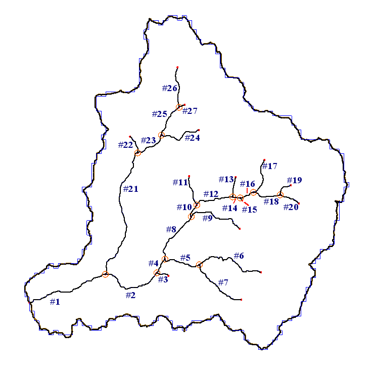
. - Double-click on arc “#1” as defined in the following figure.
- Toggle Irregular cross-section channel to enable the use of survey data.
- Click on the Define Cross Section Parameters button.
- Open the Excel® file “xsections.xls” in the Xsec_data folder.
- Copy the data for cross section #1 located in cells “A2” to “B35” (this data corresponds to cross section #1 in the following figure.
- Paste this data into the top-left cell of the WMS “XY Series Editor” spreadsheet by right-clicking on the cell and selecting “paste”.
- Select OK, then OK again.
- Double-click on arc “#2” as defined in the following figure.
- Repeat steps 4 through 9, except this time copy the data from “#2” in the Excel® spreadsheet.
- Repeat step 11 for the stream arcs #4, #8, #10, #12, #14, #16, #21, #23, #25, and #27 (we do not have survey data for all the streams).
- All streams in the basin now have either survey geometry or trapezoidal geometry for their cross sections.
- Save the GSSHA™ project by selecting the 2-D Grid Module
 .
. - Click on the GSSHA™ | Save Project File.
- Navigate to the folder you would like to save the project in.
- Enter desired project name.
- Click Save.
Just as when we set up the trapezoidal cross sections for the streams, all of the stream tools are in the Map Module.
You should now see the XY Series Editor window, which is where you will enter the cross section data (notice the spreadsheet on the left side of the window, with columns labeled “X” and “Y”). The cross section data you will be entering into this spreadsheet is located in an Excel® file, which you will copy from and paste into the “XY Series Editor”.
Contents
[hide]Adjusting the Stream Course
- If you do not already have the background image displayed, display them now by selecting File | Open…, navigating to the Judys_Branch_tutorial/Images folder, and opening all 21 carbon.jpg files. (You can filter them by typing *.jpg in the file name field before you select any.)
- Zoom in around the interchange shown in the above image.
- In the Map Module
 select the Select Feature Vertex tool
  .
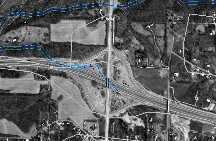
. - Adjust the vertices of the arc to be similar to the following image.
- Using the Select Feature Arc tool
 select the stream arc.
 - Select Models | GSSHA | Smooth Stream Arcs.
- Select Redistribute vertices...
- Enter 90 as the spacing value. Select OK.
- If needed, smooth the stream. Once you are done select OK.
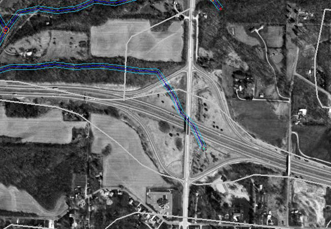
If we zoom in around the main freeway interchange we can see where the TOPAZ delineated streams do not follow the actual streams. Additionally, the natural stream course has been altered by the presence of the interchange.
We will adjust the stream course to reflect the true location of the stream.
Once the arc has been adjusted we need to make sure that the node spacing is right.
Adding an Embankment
One unique aspect of the Judy’s Branch basin is that it has a freeway bisecting it. This freeway acts as a barrier or embankment, which inhibits overland flow. To accurately model the basin, we need to take the embankment into account. The following exercise will show you how this can be done.
- Select the GIS module of WMS
 .
. - Right click on GIS Layers in the Project Explorer and select Add Shapefile Data...
- Browse to the Embankment folder, and open the EmbankmentArc.shp file.
- Click the GSSHA Coverage to make it active
- Click on the EmbankmentArc.shp file in the Project Explorer
- Select Mapping | Shapes->Feature Objects
- Click Yes to use all shapes
- Click Next, Next, and Finish to map the Embankment Arc shapefile to a GSSHA Embankment Arc.
- Toggle off the EmbankmentArc.shp file in the Project Explorer
- Open the Display Options dialog
- Click on Map Data in the left panel
- Click on the button displaying the vertex icon and change the radius to 5 and the color to yellow.
- Click OK to close the Display Options dialog.
- Click on the GSSHA coverage to view the Map Tools
- Choose the Select Feature Vertex tool.
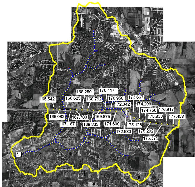
- Using Figure 27 as your guide, select each vertex of the embankment arc and assign it the corresponding elevation in the properties window on the right.
- Select the “Select Arc” tool
 .
. - Double click on the embankment arc to bring up the Feature Arc Properties window
- Click the Edit Embankment Profile button.
- View the embankment arc profile and notice the two ending points of the embankment arc are still zero.
- Click OK to close the Embankment Arc Profile Editor
- Click OK to close the Feature Arc Properties window
- Choose the Select Feature Vertex tool
- Right click on the vertex that lies on top of the node where the embankment arc meets the watershed boundary
- Select Clean
- Click OK in the Clean dialog
- The embankment arc node is hidden by the watershed boundary. Click again in the same spot as the vertex. WMS will then snap the vertex and node together.
- Repeat for the node on the opposite end of the embankment arc
- Choose the Select Feature Node tool.
- Click on the node where the embankment arc meets the watershed boundary
- For the node on the left side of the watershed, assign an elevation of 165.
- For the node on the right side of the watershed, assign an elevation of 178.
- Choose the Select Arc tool.
- Double click on the embankment arc.
- Click the Edit Embankment Profile button to view the embankment profile. Notice the profile looks much smoother now.
- Click OK, and OK to return to the WMS window
- In the 2D Grid module
 select Display | Display Options…
 - Turn on embankments and cells. Click OK.
- Zoom in on the embankment arcs.
- In the Map Module
 , zoom in on the problem spot.
 - Using the Select Feature Node
 tool select the end node on either of the arcs that do not connect.
 - Right-click on the selected node, select the clean command, make sure the option to snap selected nodes is on, and select OK.
- At the lower left corner of the screen, you are prompted to select a snapping point. You should select the end point of the other arc for snapping. After selecting this point, the arcs will snap together.
- Select the Refresh button
 to update the display of your embankment cells.
You should see the embankment arc running across the center of the watershed. Although the embankment arc is shown in its proper geographic location, the elevations at each vertex need to entered manually. We'll adjust the vertex display settings to see them better.
Since we created the embankment arc using a shapefile, the embankment arc nodes did not snap to the watershed boundary. First we'll snap the embankment arc to the watershed boundary, then we'll assign elevations at the two nodes.
WMS uses the embankment arc to define cells edges as overland flow barriers. You can view these cell edges in the Display Options dialog .
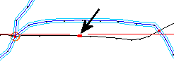
You should see the cell edges nearby highlighted in red. These red edges are the actual embankments that GSSHA™ uses. If there are any gaps in the embankment edges, you will need to adjust the embankment arcs accordingly. Note, if the embankment arc, a black line by default, coincides with one of the cell edges it may appear that the line is broken when in fact it is continuous. An example of this is shown in the second image below. If the embankment arc is broken, an entire cell will lack the red highlighting. For example, if you see a problem similar to the first image below. (if you have done everything correctly, you will probably not need to do this):
It is because the embankment arcs are not snapped together or do not extend far enough. To fix the problem:
Adding Structures
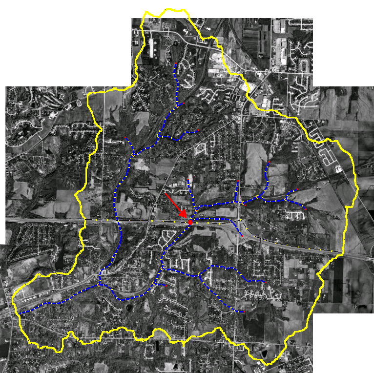
Due to the embankment we created in the previous exercise, water from the top half of the model will only be able to reach the outlet by flowing through the streams that pass through the embankment. To control the amount of water that passes through the stream at the embankment we will create a structure (in this case a culvert), at a node where the stream arcs intersect the embankment. The following steps outline how this is to be done.
- Select the map module
 .
. - Pick the Select Feature Point/Node tool
 .
. - Using the figures below as a reference, double-click on the point (node) where the two streams intersect and cross the highway.
- In the “Node Type” section of the Feature Node Attributes dialog, click on the drop down box and select Link Break.
- In the Hydraulic Structure and Curves section of the Feature NodeAttributes dialog, click on the Culvert button to add
- Click on the word “Culvert 1” that appears in the text box below “Hydraulic Structures and Curves”.
- Select the drop-down box next to culvert type and select “Rectangular”.
- Enter the following values to define the culvert:
- Click OK.
| |||||||||||||||||||
Once you have finished the culvert, save the model and run it.
GSSHA Tutorials
GSSHA Tutorial Download Website
