Tutorials:16 Simple Constituent Transport
This tutorial is compatible with:
- WMS Version 8.2 and later
- GSSHA Version 5.0 and later
Disclaimer: GSSHA tutorial exercises do not represent real world conditions
Two types of reactive constituent transport are available in GSSHA. As explained in the GSSHA wiki, constituents can be simulated as simple first order reactants. The nutrient cycle can also be simulated with the Nutrient Simulation Model (NSM). In either case, the overall simulation methods within the GSSHA model are the same. Only the rates of mass absorption and decay are different. It is then possible to simulate nutrients as simple constituents, as well as simulating them with the full nutrient cycle. Use of first order constituents requires that the user have explicit information about the contaminants being simulated as the user must supply all the reaction rates for the model. On the other hand, when using NSM many different reactions occur and most of the reaction rates are calculated by NSM. There is no limit as to the number of simple constituents that can be simulated at one time. In this tutorial, two contaminants will be simulated.
Open the Base Model
- In the 2D Grid Module
 select GSSHA™ | Open Project File.
 - Browse to the Judy's_Branch_tutorial/Contaminant_Transport directory and open the file named Contaminants.prj.
- In the 2D Grid Module select GSSHA™ | Save Project File.
- Browse to the Judy's_Branch_tutorial/Contaminant_Transport/Personals directory and save the file as Contaminant_Transport.prj.
This base model has already been set as a long term simulation model with precipitation data and meteorological data for one week. If you have questions on how to set a long term simulation model, please refer to the Long Term Simulations Tutorial.
Adding Contaminants
Constituent transport can be simulated on the overland flow plane, in the channel network including reservoirs, and in the soil column. These parameters are added in different dialog boxes in GSSHA as shown in the steps below.
- Make sure that your project has 12 coverages,9 of which should be rainfall events. GSSHA™ should be the active coverage in the Project Explorer as shown in Figure 1 below.
- Select the 2D Grid Module if not already selected. Go to GSSHA™ | Job Control.
- In the dialog box that opens, click on the box beside Contaminant Transport to select this option. Make sure that Long Term Simulation is also selected. See Figure 2.
- Click on the Edit parameter button for Contaminant Transport. In the dialog box that opens, click on the add button to add two contaminants and enter the information found in Table 1. Click OK.
 |
 |
The base output file column specifies the location of the output files that will be generated for each contaminant. Make sure the location for contaminant1 and contaminant2 is as follows:
- \Judy's_Branch_tutorial\Contaminant_Transport\Personals\Contaminant1
- \Judy's_Branch_tutorial\Contaminant_Transport\Personals\Contaminant2
| Description | Index Map | Precipitation Concentration (mg/L) | Partition |
|---|---|---|---|
| Contaminant 1 | Land Use | 0.0 | 0.5 |
| Contaminant 2 | Land Use | 0.0 | 0.4 |
This is the first step in parameter input. This information will help populate the mapping table with the number of contaminants that will be simulated. Notice that in the index map column you had the option of choosing between Uniform, Land Use, Soil Type and Combined Index Maps. The index map you use will depend on the nature of your model. The Uniform Index map can be used just to set up your model and make sure it is working as it simplifies the setup, but it does not necessarily represent real conditions. The use of the other three Index Maps will depend on the nature of the contaminants you are simulating. This requires that you know your project really well. In this tutorial we will use the Land Use Index Map. We will assume that a certain area of our watershed is contaminated by either point or non-point sources. This could be a landfill, or areas that receive runoff and/or leachate from agricultural activities, residential areas or from mining and logging operations.
Before entering the needed parameters in the mapping table we will define the contaminant conditions for the channel network.
- In the Job control Dialog box that is still open, make sure that Diffusive Wave is selected. Click on Edit Parameters. A dialog box will show up as shown on Figure 3.
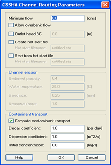
Figure 3 -
- Select Compute Contaminant Transport and enter the following values:
decay coefficient: 1.0
dispersion coefficient: 1.0
Initial Concentration: 0.0
- Click OK. This will define the conditions in the channel network.
- Click OK to close the job control dialog box.

With the 2D grid as your active module, go to GSSHA™ | Map Tables. Values for Roughness, Evapotranspiration, Infiltration and Initial Moisture should already be defined. We will now fill in the values for Contaminants.
- Click on the Contaminants Tab. From the Index Map Drop down Menu select “Land Use”.
- From the Contaminant Drop down Menu select each contaminant and click Generate IDs. You will have five columns of values for each contaminant. Input the values from Table 2 and Table 3 respectively:
- Click OK
| Parameters | Contaminant 1 | ||||
|---|---|---|---|---|---|
| LU 11 | LU 14 | LU 16 | LU 21 | LU 41 | |
| Dispersion (m2/s) | 0 | 0 | 0 | 0 | 0 |
| Decay (d-1) | 1 | 1 | 1 | 1 | 1 |
| Uptake (m/day) | 1 | 1 | 1 | 1 | 1 |
| Mass loading (kg/cell) | 100 | 0 | 0 | 0 | 0 |
| Groundwater concentration (mg/L) | 1 | 0 | 0 | 0 | 0 |
| Initial Concentration (mg/L) | 0 | 0 | 0 | 0 | 0 |
| Soil water distribution coefficient (L/kg) | 0.5 | 0.5 | 0.5 | 0.5 | 0.5 |
| Max concentration/ solubility-Cmax (mg/L) | 100000 | 100000 | 100000 | 100000 | 100000 |
| Parameters | Contaminant 2 | ||||
|---|---|---|---|---|---|
| LU 11 | LU 14 | LU 16 | LU 21 | LU 41 | |
| Dispersion (m2/s) | 0.5 | 0.5 | 0.5 | 0.5 | 0.5 |
| Decay (d-1) | 0.8 | 0.8 | 0.8 | 0.8 | 0.8 |
| Uptake (m/day) | 1.5 | 1.5 | 1.5 | 1.5 | 1.5 |
| Mass loading (kg/cell) | 200 | 0 | 0 | 0 | 0 |
| Groundwater concentration (mg/L) | 0 | 0 | 0 | 0 | 0 |
| Initial Concentration (mg/L) | 0 | 0 | 0 | 0 | 0 |
| Soil water distribution coefficient (L/kg) | 0.4 | 0.4 | 0.4 | 0.4 | 0.4 |
| Max concentration/ solubility-Cmax (mg/L) | 100000 | 100000 | 100000 | 100000 | 100000 |
Populating the mapping tables in this way is telling WMS that only the Land Use 11 has contaminant loading. The rest of the watershed has been assigned values of zero.
Let’s take a look at the parameters required to simulate contaminant transport. Dispersion refers to the mixing that occurs because the porous media forces some solute molecules to move faster than others while following a tortuous path through pores of different sizes (1). It is caused by variation in velocities and it can be vertical, lateral and longitudinal. Typical values of dispersion coefficient (m2/sec) can range from 10-3 to 10-1 (vertical), 10-2 to 100 (lateral) and 10-1 to 104 (longitudinal). (2)
The Decay coefficient (Kd) represents the production or decay of solute concentration within the porous medium. It is a rate constant that represents increasing concentration when it is negative in value and decreasing concentration when it is positive. (3) Examples of values for some constituents are found in Table 4.
| Constituent/Process | Decay Coefficient (d-1) |
|---|---|
| Anammox (4) | 0.0048 |
| benzene (5) | 0.0046 |
| Coliform bacteria (6) | 2—4 |
| BOD5 (6) | 0.2—0.5 |
| Nutrients (6) | 0.1—0.25 |
We understand uptake (Ku) to be the incorporation or absorption of a constituent such as a nutrient by a medium (or a tissue if when referring to organisms), and its permanent or temporary retention. Examples of uptake coefficient values are found in Table 5.
| Constituent | Uptake Coefficient |
|---|---|
| OH and HO2 on water (7) | 0.01—1 |
| OH and HO2 on sulfuric acid (7) | 0.008—0.03 |
| O3 on water (7) | 0.0008 |
| I2 on aqueous surfaces (8) | (3.7 ± 2.0) x 10-4 |
| Note: the GSSHA wiki has uptake with units of m/day as specified on this page | |
The mass loading (kg/cell) refers to the amount of contaminant present in the overland cell. If we are simulating contaminant transport within the soil column, then the mass loading refers to the mg of contaminant per kg of soil.
The initial concentration values asked for in the mapping table refer to the concentration of constituents in a water surface, or in other words, the hot start concentration.
The soil water distribution coefficient (Kd) also known as partition coefficient is a direct measure of the partitioning of a contaminant between the solid and aqueous phases. (9) Table 6 has partition coefficients for lead in different media combinations, obtained from the EPA site.
| Soil Description | pH | Kd (mL/g) |
|---|---|---|
| Sediment, split rock formation | 4.5 | 100 |
| 7.0 | 4,000 | |
| Sand | 4.5 | 280 |
| Sandy Loam | 7.5 | 3,000 |
| 8.0 | 4,000 | |
| Loam | 7.3 | 21,000 |
| Organic Soil | 5.5 | 30,000 |
As you can see, modeling first order constituents require that you have a thorough knowledge of your contaminant and modeling area as you are required to input the coefficients previously described.
Our model has all the required inputs to simulate contaminants. We are ready to run the model.
Save and Run the Contaminants Model
- In the 2D Grid Module select GSSHA™ | Save Project File.
- Save the file as Contaminant_Transport.prj
- When prompted to replace the existing file, click yes.
- Select GSSHA™ | Run GSSHA™.
- When GSSHA™ is done running, make sure the option to Read solution on exit is toggled on and click Close.
View Results
There are several different outputs generated when running the model. In the outlet location, you should get two constituent graph solutions, one for Constituent Mass and one for Constituent Concentration.
- In the Project Explorer, right-click on the Outlet Constituent Mass graph, located below the GSSHA™ solution folder (the folder with the letter "S" on it)
- Select View Graph. You have the option of selecting the contaminant you want to view. The plot window should show a graph similar to the one in Figure 4.
- Close the contaminant plot.
- You can follow the same steps for Constituent Concentration graph. A plot for the concentration of both contaminants is shown in Figure 5.


To view overland contaminant mass and concentration, do the following:
- In the 2D Grid module select Display | Display Options
- Turn on the 2D Grid Contours.
- Select OK.
- In the data tree, right-click on mass_01 under the solution folder.
- Select Contour Options.
- Under Contour Method select 'Color Fill.'
- Click on Color Ramp. A dialog box as shown in Figure 6 will appear. Click the Reverse button.
- Select OK.
- In the mass_01 Contour options dialog, the number of contours should be defaulted to 20. Reduce this number to 10.
- In the Contour Method drop down menu that is defaulted as ‘use Color Ramp’, select ‘Specify each color’.
- You will note that the colors have now a drop down menu. Change your first color from blue to white. Leave the rest as they are. See Figure 7
- Click OK to exit the dialog box.
- Right-click on mass_01 in the data tree.
- Select Contour Options.
- Turn on the legend.
- Click OK. Your mass overland display for contaminant 1 (08/24/01 at 9:45 am) should look something like this:
- You can follow steps from 4-15 if you want to visualize mass_02, conc_01 or conc_02 as well.


A set of time steps appear in the right pane of your WMS window as you selected mass_01. Click around on a few of them between 7:00-10:00 a.m. on 08/24/2001. It would be helpful if we knew what the colors represented.

In order to visualize mass and contaminant concentrations along the stream network, we need to turn on the contours for the 2D Scatter Data.
- In the project explorer, right click the
 Link/node icon. Select the Display Options dialog.
 - Turn on the contours for the 2D Scatter Data.
- Select a radius and Z Magnification (try a radius of 4 and a Z magnification of 50). If the lines are too big, you might need to decrease the Z magnification.
- Click OK.
- Select either the Contaminant mass or the Contaminant conc. data set in the 2D Scatter Data folder in the data tree.
- Select a time step other than the first one in the Properties window, such as 08/24/2001 between 7:00-10:00 am.
- If you rotate into 3D mode
 , or change from plan view
  to perspective view
  , you will see the lines representing stream mass. In the properties folder you will see the time steps. As you select individual time steps the data for that time step both the 2D grid data and the 2D scatter data will be contoured.
Your display for contaminant mass on the stream network (08/24/2001 9:45 am) should look something like this:

Even when behavior of contaminants in the soil column is not graphically displayed in WMS, we can open the summary file and get information on this and the rest of the processes simulated.
- Double-click on Summary File under the solution folder.
- If WMS asks for your editor just click OK.
- Look through the summary file. Notice the kinetics of overland, stream and soil column contaminant transport. It is also good to check things like mass balance and the volume remaining on the surface.
- When you are done you can close the window.
This concludes the GSSHA™ constituent transport tutorial.
References
(2) Ecosystems Research Division. WASP7 Course. Environmental Protection Agency. http://www.epa.gov/athens/wwqtsc/courses/wasp7/
(3) Modeling the Environmental Fate of Microorganisms. Christon J. Hurst. 1991 http://books.google.com/books?id=TMgoX86EIZIC&pg=PA30&lpg=PA30&dq=contaminant+decay+coefficient+K&source=bl&ots=3KrR2ex-JY&sig=akvyOWf6ZH1JqonIaulACZQpFrs&hl=en&ei=oPVcSsaZEILusgONru2lCg&sa=X&oi=book_result&ct=result&resnum=1
(4) Experimental Determination of Anammox Decay Coefficient. D. Scaglione et.al. Journal of Chemical Technology and Biotechnology. Vol 84. Issue 8. 1250-1254. http://www3.interscience.wiley.com/journal/122267762/abstract
(5) Bioremediation and Natural Attenuation. Pedro J. J. Alvarez, Walter Arthur Illman. 2005 http://books.google.com/books?id=fSUtC8luIp0C&pg=PA196&lpg=PA196&dq=decay+coefficients&source=bl&ots=yRW20vQ_UW&sig=3GsPXKt2r9Vb2h_U7fV_PIQfxSU&hl=en&ei=kjJWSu2KDpDWtgOOqK3PDg&sa=X&oi=book_result&ct=result&resnum=6
(6) Water Resources and Natural Control Processes. Lawrence K. Wang, Norman C. Pereira. 1987. http://books.google.com/books?id=lR2DeuTrTsMC&pg=PA62&lpg=PA62&dq=simple+and+reactive+constituents&source=bl&ots=aGp9KEYkJA&sig=LVZEF_OjSao0jkpjKCs0BhuX1K4&hl=en&ei=bC9WSvbwIYrasQOeqKX0AQ&sa=X&oi=book_result&ct=result&resnum=6
(7) Interpretation of Uptake Coefficient Data Obtained with Flow Tubes. E. James Davis J. Phys. Chem. A, 2008, 112 (9), pp 1922–1932. February 12, 2008 http://pubs.acs.org/doi/abs/10.1021/jp074939j
(8) The Uptake Coefficient of I2 on Various Aqueous Surfaces. Takami Akinori et.al. Journal of Atmospheric Chemistry. ISSN 0167-7764. 2001, vol. 39, no2, pp. 139-153. http://cat.inist.fr/?aModele=afficheN&cpsidt=1095928
(9) http://www.epa.gov/rpdweb00/docs/kdreport/vol2/402-r-99-004b_appf.pdf
(10) http://www.epa.gov/rpdweb00/docs/kdreport/vol2/402-r-99-004b_appf.pdf
GSSHA Tutorials
GSSHA Tutorial Download Website