Template:GUM9
9 - Continuous Simulations
GSSHA can be used to perform continuous simulations by specifying the LONG_TERM card in the project file, and providing the necessary input data. Continuous simulations require that one of two optional methods for calculating evapo-transpiration (ET) be selected, Deardorff (1978) or Penman-Monteith (Monteith, 1965, 1981), as described in Section 9.1. Hourly hydrometeorological observations are required for either method. The file containing the hourly values of hydrometeorological values is specified with the HMET_TYPE card. The TYPE can be WES, SAMPSON, or SURFAWAYS, as described in Section 9.3. The hydrometeorological inputs are used to compute potential evapo-transpiration (PET) with one of two ET methods. This PET is then sent to the chosen soil moisture accounting method as a demand. The amount of the demand that can be satisfied is the actual ET (AET). The AET is met based on the soil hydraulic properties, soil mositure, balance with other sources (infiltration, flow from groundwater) and demands (drainage). Anytime long-term simulations are performed snowfall accumulation and melting are also calculated, Section 9.2. To perform long term simulations, infiltration must be calculated with either GAR or RE by use of the INF_REDIST or INF_RICHARDS cards, respectively. In GSSHA v5 and above the multi-layer GA model can also be used for continuous simulations. Multi-layer GA is specified with the INF_LAYERED_SOIL card. When the GAR or multi-layer GA method of infiltration is specified, soil moistures are calculated with a two layer soil moisture model, as described in section 9.2. When RE is chosen, soil moisture is calculated as part of the overall solution.
9.1 Computation of Evaporation and Evapo-transpiration
The evaporation and evapo-transpiration models incorporated in GSSHA allow calculation of the loss of soil water to the atmosphere, improving the determination of soil moistures. Two different evapo-transpiration options are included:
- bare-ground evaporation from the land-surface using the formulation suggested by Deardorff (1978), and
- evapo-transpiration from a vegetated land-surface utilizing the Penman-Monteith equation (Monteith, 1965, 1981).
Variants of these two representations are widely used in land-surface schemes of climate and distributed hydrologic models (e.g., Dickinson et al., 1986; Beven, 1979).
To accurately compute fluxes of soil water to the atmosphere, energy fluxes between the atmosphere and the ground must first be computed. These energy, or radiation, fluxes, discussed in Section 9.1.1, are the forcing terms in the evapo-transpiration calculations. Ground temperature is an important component in both the Deardorff and Penman-Monteith formulations, and the fluxes computed in Section 9.1.1 are used in the computation of the ground temperature as described in Section 9.1.2. A detailed presentation of the Deardorff method in Section 9.1.3 describes how the computed fluxes and ground temperatures can be related to bare-soil evaporation. Section 9.1.4 details how the computed fluxes are adjusted and applied for computation of evapo-transpiration with the Penman-Monteith equation. Finally, Section 9.1.5 describes the additional inputs needed for ET calculations.
9.1.1 Computation of Auxiliary Energy and Heat Fluxes
Realistic estimates of incoming and outgoing radiation fluxes are needed for accurate estimates of ET. The important components of the energy budget are long-wave radiation, discussed in Section 9.1.1.1, short wave radiation, discussed in Section 9.1.1.2, and heat conduction into the soil, Section 9.1.1.3. Influences of soil, water, vegetation and cloud albedos, atmospheric emissivities, and sloping-terrain effects on energy fluxes must be included in the calculations. The effects of albedos and emissivities are of great importance in determining radiation fluxes and warrant detailed representation (Pielke, 1984).
9.1.1.1 Net Incoming Short-wave Radiation
The net incoming short-wave radiation can be represented as:
-
 (53)
(53)
where: A is the albedo, and Rs, direct and Rs, diffuse are direct and diffuse contributions of short-wave radiation, respectively.
It is also imperative that short-wave energy influxes be modified to account for sloping terrain effects. As described by Young (1972), even in the Great Plains region of North America (one of the flattest places on earth), only 7% of the land area can be classified as flat in relation to solar radiation calculations. Despite the significance of terrain, most hydrologic and Global Climate Model (GCM) land-surface schemes ignore the sloping terrain effects when estimating the soil energy budgets. Pielke (1984) found substantial differences between the solar radiation values from north and south facing slopes. Pielke and Mehring (1977) found that “the eastern slope of a 1-km mountain (with a slope of about 2°) to be about 1° to 2°C warmer in the morning and cooler by the same amount in the afternoon than the same location in the western slope.” The direct incoming solar irradiance can be represented as:
-
 (54)
(54)
where: λ is angle of incoming radiation, ζ is the local land surface slope in the azimuthal direction of the sun, and Rs, horiz,direct,ground is the direct radiation on a horizontal ground surface, computed as:
-
 (55)
(55)
where: the transmission coefficient, Kt (dimensionless) is a function of density, type and condition of vegetation, N is the fraction of sky covered by cloud cover (0-1), n is a turbidity factor of air that varies from 2.0 (clear air) to 5.0 (smoggy urban areas), currently fixed at a value of 2.0 in the code. K is the fraction of cloudless sky insolation received on a day with overcast skies, and is given as:
-
 (56)
(56)
where z is the height to the cloud-base (km), fixed in the current formulation at 1.5 km. The molecular scattering coefficient, a, is defined as:
-
 (57)
(57)
The optical air mass, m, is calculated as:
-
 (58)
(58)
where: λ is the angle from the observer’s horizon to the center of the solar disk, and is often referred to as the “solar elevation angle”. Calculation of λ is discussed below.
If no measurements of Rs,horz,direct are available, then they may be estimated based on the time of day and year, and the location of the watershed from:
|
|
 , if λ < 90°, and , if λ < 90°, and |
(59a) | |
|
|
|
(59b) |
where the solar constant, So, has a value of 1376 W m-2 (Hickey et al., 1980). Following Paltridge and Platt (1976) the ratio of the actual earth-sun distance squared (a2) to the average earth-sun distance squared (r2) on any given Julian day m* can be estimated using the following relationship (60):
where:
-
 (61)
(61)
where: m* is the number of the day [i.e., ranging from 0 (January 1) to 364 (December 31)], and do is the Julian day fraction of the year converted to radians. The angle (i) between the direct solar radiation and the normal to the slope is defined as (Kondrat’yev, 1969) :
-
 (62)
(62)
The slope of the terrain (α) is given by:
-
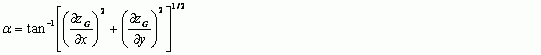 (63)
(63)

where: ∂zG/∂x and ∂zG/∂y represent the incremental slopes in the x and y directions. The zenith angle (λ) is defined by:
-
 (64)
(64)
where: angle φ is the latitude at the site of interest. The orientation of the sun’s azimuth β relative to the azimuth of the terrain slope γ is given by β–γ. The trigonometric relationship for γ is:
-
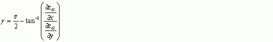 (65)
(65)

The trigonometric relationship for β is:
-
 (66)
(66)
where: δsun is the declination angle of the sun (varying between +23.5? on June 21 to -23.5? on December 22), and can be obtained by using the following formulation (Paltridge and Platt, 1976):
-
 (67)
(67)
where: δsun is in radians. The hour angle, hr (0°≡noon) is represented mathematically when the sun is east of the observer’s longitude as follows (Curtis and Eagleson, 1982):
-
 (68)
(68)
where: Ts is the standard time at the site of interest (counted from midnight; i.e. from 0.00 to 23.59), ΔT2 is the difference between true solar time and mean solar time in hours (small; hence is neglected in this analysis), and ΔT1 is the difference between the standard and local longitudes (in hours) given as:
-
 (69)
(69)
where i* = 1 for longitudes located to the east of Greenwich and i* = -1 for those located to the west, and θS and θL are the longitudes of the standard- and the observer-meridian, respectively. The standard-meridian is defined as the meridian where the observer’s time zone is centered. When the sun is west of the observer’s longitude the following relationship is used:
-
 (70)
(70)
The diffuse short-wave radiation is obtained by using the following relationship (Kondrat’yev, 1965):
-
 (71)
(71)
Lee (1978) noted that the difference between Rs,diffuse and Rs,horiz.,diffuse is only 2% for slopes less than 30%. Lee (1978) also showed that for slopes less than 36%, the contribution to the total solar radiation by the reflection of total solar from surrounding sloped terrain is only 3% or less. The diffuse horizontal radiation, Rs,horiz.,diffuse data are extracted from NOAA-NREL CD-ROMs, and hence atmospheric scattering and absorption effects are neglected.
9.1.1.2 Net Incoming Long-wave Radiation
The net incoming long-wave radiation can be represented as follows:
-
 (72)
(72)
where: A is the long-wave surface albedo, σ is the Stephan-Boltzmann constant with a value of 5.67 x 10⁻⁸ Jm-2s-1K-4, Tg and Ta are the absolute ground and the air temperatures (Kelvins), respectively, K* is the cloudiness-correction factor (dimensionless), and Ea and Eg are the emissivities of the air and the ground surfaces, respectively (dimensionless). Following Bras (1990), it is assumed that the ground surface acts as a blackbody, with an emissivity of 1.0. The long-wave radiation from clear skies is strongly related to the atmospheric water content. The following formulation is used to evaluate the atmospheric emissivity (Idso, 1981):
-
 (73)
(73)
where e is the vapor pressure (mb), and can be obtained from the following relationship:
-
 (74)
(74)
where: rh is the relative humidity (dimensionless, expressed as a decimal number between 0 and 1), and es is the saturated vapor pressure (mb). Using the Teten’s formula (Teten, 1930) the saturated vapor pressure can be approximately evaluated as:
-
 (75)
(75)
The presence of clouds gives rise to an increase in long-wave radiation. The following relationship, suggested by the TVA (1972), is used to evaluate K*:
-
 (76)
(76)
where N is the fraction of sky covered by clouds.
9.1.1.3 Heat Conduction into the Soil
Many models neglect the soil heat flux (Manabe et al., 1974; Gates, 1974), however, Deardorff (1978) has found the assumption of an insulated soil surface to be especially poor under random atmospheric forcing-conditions. Following Kasahara and Washington (1971), in GSSHA the soil heat flux at the surface (positive when directed into the soil) is represented as a function of sensible heat flux. Deardorff (1978) found the following relationship to be of “intermediate but surprisingly acceptable accuracy” in determining the sum of energy fluxes into the soil (W m-2) for short time-steps:
-
 (77)
(77)
where Hs is the sensible heat flux (W/m2) (positive when directed upward), represented mathematically as:
-
 (78)
(78)
where: cp is the specific heat at constant pressure, equal to 1.013 kJ kg-1 °C-1, ua is the wind speed (m/s) at the reference level, z, and cH is the dimensionless heat or moisture transfer coefficient applicable to bare soil. Following Deardorff (1978) a value of 0.0025 is selected for cH. The air density ρa is calculated as (kg m3):
-
 (79)
(79)
where: Pa is the atmospheric pressure in kPa, and Ta is the air temperature in °C.
9.1.2 Estimation of Ground Temperature
Because ground temperature appears explicitly in the outgoing long-wave energy flux-term, and implicitly in the Deardorff (1978) and Penman-Monteith evaporation formulae, it is important for radiation and evaporation calculations. Ground temperature varies considerably during the diurnal cycle and is not generally measured or provided by meteorological or weather stations. In GSSHA the ground temperature is obtained numerically by solving the surface energy balance equation with the Newton-Raphson iterative method as described by Deardorff (1978).
Assuming that the energy lost due to temporary storage, advection and biochemical usage are negligible for non-vegetated surfaces, the surface energy balance formulation can be written as:
![]() (80)
(80)
where: the terms Hs, Rl, Rs and G have been previously defined, and E is the evaporation latent heat flux (W/m2) from bare soil, as described in Section 9.1.3.
The saturation specific humidity (kg/kg), a function of ground temperature, qsat (Tg) (mb) can be calculated from:
![]() (81)
(81)
where: ε is the ratio of molecular weight of water vapor to that for dry air (0.622), and qa is the specific humidity, estimated by substituting e = rhes for es, where rh is the relative humidity.
The Clausius-Clapeyron equation is used to calculate the derivative of qs with respect to Tg as:
![]() (82)
(82)
where: Rwater is the gas constant for water vapor (461 J kg-1 °K-1) and L is the latent heat of evaporation (2.50036 MJ kg-1). Following Williamson et al. (1987), the latent heat of evaporation, known to vary with ground temperature, is a constant. The ground temperature can be obtained iteratively using the following relationship:
![]() (83)
(83)
where: K indicates the iteration count, ƒ(Tg) is obtained from Equation (80) and ƒ’ (Tg) is obtained from Equation (82). The initial value for the iterative procedure is the surface temperature from the previous time step, Tgn-1. The procedure is repeated until the following condition is satisfied:
![]() (84)
(84)
A convergence criterion, δe of 0.001 °K is utilized in this analysis. When the convergence criterion is satisfied the Clausius-Clapeyron equation is solved, and Tgn = Tgk+1.
9.1.3 Evapo-transpiration
Evaporation from a bare surface can be computed using the Deardorff equation by specifying the ET_CALC_DEARDORFF card in the project file. When using the Deardorff method only the physical components of evaporation are considered. Plants are not considered. Compared to the Penman-Montieth method (1971), use of the Deardorff method can result in higher evaporation and lower soil moistures because residual soil moisture is the lower limit on soil moisture and resistance of the plant canopy to evaporation is not considered. The Deardorff method is not appropriate in vegetated areas and have limited applicability. Inputs to the mapping table for ET calculations, described below, are the same for the two methods.
The ET_CALC_PENMAN project card is used to select the Penman-Monteith method for evapo-transpiration. The Penman-Monteith equation is one of the most advanced resistance-based models available for the prediction of evapo-transpiration from a vegetated land-surface (Shuttleworth, 1993). Although Monteith (1965) points out several simplifying assumptions utilized to derive the Penman-Monteith evaporation formula, Lemeur and Zhang (1990) have found that for arid watershed the performance of the Penman-Monteith is better than both the CRAE (Morton, 1983) and the Advection-Aridity (Brutsaert and Stricker, 1979) models. In the Penman-Monteith model, the potential evapo-transpiration estimates are obtained by using the following relationship:
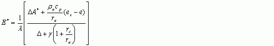 (85)
(85)

where:
- Δ is the slope of the specific humidity/temperature curve between the air temperature and the surface temperature of the vegetation (kPa °C-1)
- λ is the latent heat of vaporization of water (2.50036 MJ/kg)
- cp is the specific heat of air at constant pressure (1.013 kJ kg-1 °C-1)
- γ is the psychrometric constant kPa °C-1)
- ra is the aerodynamic resistance to the transport of water vapor from the surface to the reference level z (s/m)
- rc is the (Monteith) canopy resistance (s/m) to the transport of water from some region within or below the evaporating surface to the surface itself. The canopy resistance is expected to be a function of the stomatal resistance of individual leaves. Under wet-canopy conditions rc = 0.
- A* is the available energy given by A* = (Rl + Rs) - G (W/m2)
- Rs is the net incoming short-wave radiation at the reference level z, (W/m2) Section 9.1.1.1.
- Rl is the net long-wave radiation at the reference level z, (W/m2) Section 9.1.1.2.
- G denotes the sum of energy fluxes into the ground, to adsorption by photosynthesis and respiration and to storage between ground level and z (in W/m2), Section 9.1.1.3.
The standard reference level, z, is taken as 2 m. The current formulation does not explicitly calculate the leaf temperature of the vegetation canopy, and the ground temperature is substituted for the leaf temperature when calculating Δ. The psychrometric constant, γ, is defined as:
 (86)
(86)
where: P is the atmospheric pressure (kPa). The gradient of the saturation vapor pressure curve with respect to temperature, Δ, is given by:
 (87)
(87)
The rate of water diffusion from the ground surface due to turbulence is controlled by the aerodynamic resistance term, ra. This term is a function of wind speed and the height of the vegetation cover. Mathematically, ra is represented as:
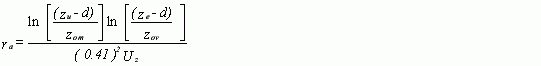 (88)
(88)

where: zu and ze are the heights of the wind speed and humidity measurements (m), respectively, and Uz is the wind speed (m/s). Following Brutsaert (1975), zom is assumed to be 0.123hc and zov is assumed to equal 0.0123hc, where hc is the mean height of the crop (m). According to Monteith (1981) d = 0.67 hc.
9.1.4 Parameter Values
Calculation of evapo-transpiration requires additional parameter values be assigned to every active grid cell. These parameters may be assigned with either the Mapping Table File, Section 11, or GRASS ASCII maps specified with project cards described in Section 3.8. ET parameters are typically assigned with a combination soil texture/land use (STLU) index map. The Deardorff method requires values of land surface albedo. For the Penman-Monteith method, values of land surface albedo, vegetation height, vegetation canopy resistance, and vegetation transmission coefficient are needed.
9.1.4.1 Land Surface Albedo
Ground surface temperature calculations, discussed in Section 9.1.2, require values of land surface albedo, which describe the fraction of long-wave radiation reflected back to the atmosphere. Values range from 0.0 to 1.0. Literature values for a variety of land covers compiled from a number of sources are listed in Table 11.
| Ground Cover | Albedo |
|---|---|
| Fresh Snow | 0.75 - 0.95b, 0.70 - 0.95c, 0.80 - 0.95d, 0.95e |
| Fresh snow (low density) | 0.85f |
| Fresh snow (high density) | 0.65f |
| Fresh dry snow | 0.80 - 0.95g |
| Pure white snow | 0.60 - 0.70g |
| Polluted snow | 0.40 - 0.50g |
| Snow several days old | 0.40 - 0.70b, 0.70c, 0.42 - 0.70d, 0.40e |
| Clean old snow | 0.55f |
| Dirty old snow | 0.45f |
| Clean glacier ice | 0.35f |
| Dirty glacier ice | 0.25f |
| Glacier | 0.20 - 0.40e |
| Dark soil | 0.05 - 0.15b, 0.05 - 0.15g |
| Dry clay or gray soil | 0.20 - 0.35b, 0.20 - 0.35g |
| Dark organic soils | 0.10f |
| Dry black soil | 0.14i |
| Moist black soil | 0.08i |
| Dry gray soils | 0.25 - 0.30i |
| Moist gray soils | 0.10 - 0.20g, 0.10 - 0.12i |
| Dry blue loam | 0.23i |
| Moist blue loam | 0.16i |
| Desert loam | 0.29 - 0.31i |
| Clay | 0.20f |
| Dry clay soils | 0.20 - 0.35d |
| Dry light sand | 0.25 - 0.45b |
| Dry, light sandy soils | 0.25 - 0.45g |
| Dry, sandy soils | 0.25 - 0.45a |
| Light sandy soils | 0.35f |
| Dry sand dune | 0.35 - 0.45b, 0.37c |
| Wet sand dune | 0.20 - 0.30b, 0.24c |
| Dry light sand, high sun | 0.35f |
| Dry light sand, low sun | 0.60f |
| Wet gray sand | 0.10f |
| Dry gray sand | 0.20f |
| Wet white sand | 0.25f |
| Dry gray sand | 0.35f |
| Yellow sand | 0.35i |
| White sand | 0.34 - 0.40i |
| River sand | 0.43i |
| Bright, fine sand | 0.37i |
| Rock | 0.12 - 0.15i |
| Peat soils | 0.05 - 0.15d |
| Dry black coal spoil, high sun | 0.05f |
| Dry concrete | 0.17 - 0.27b, 0.10 - 0.35e |
| Road black top | 0.05 - 0.10b |
| Asphalt | 0.05 - 0.20e |
| Tar and gravel | 0.08 - 0.18e |
| Densely urbanized areas | 0.15 - 0.25i |
| Urban area | 0.10 - 0.27 with an average of 0.15e |
| Long grass (1 | 0 m) 0.16e |
| Short grass (2 cm) | 0.26e |
| Wet dead grass | 0.20f |
| Dry dead grass | 0.30f |
| High, dense grass | 0.18 - 0.20i |
| Green grass | 0.26i |
| Grass dried in sun | 0.19i |
| Typical fields | 0.20f |
| Dry steppe | 0.25f, 0.20 - 0.30g |
| Tundra and heather | 0.15f |
| Tundra | 0.18 - 0.25e, 0.15 - 0.20g |
| Heather | 0.10i |
| Meadows | 0.15 - 0.25g |
| Cereal and tobacco crops | 0.25f |
| Cotton, potatoes and tomato crops | 0.20f |
| Cotton | 0.20 - 0.22i |
| Cotton plantations | 0.20 - 0.25g |
| Potatoes | 0.19i |
| Potato plantations | 0.15 - 0.25g |
| Lettuce | 0.22i |
| Beets | 0.18i |
| Sugar Cane | 0.15f |
| Orchards | 0.15 - 0.20e |
| Agricultural crops | 0.18 - 0.25e, 0.20 - 0.30d |
| Rice field | 0.12i |
| Rye and wheat fields | 0.10 - 0.25g |
| Spring wheat | 0.10 - 0.25i |
| Winter wheat | 0.16 - 0.23i |
| Winter rye | 0.18 - 0.23i |
| Deciduous forests - bare of leaves | 0.15e |
| Deciduous forests - leaved | 0.20e |
| Deciduous forests | 0.15 - 0.20g |
| Deciduous forests - bare with snow on the ground | 0.20d |
| Mixed hardwoods in leaf | 0.18f |
| Rain forest | 0.15f |
| Eucalyptus | 0.20f |
| Forest - pine, fir, oak | 0.10 - 0.18c |
| Forest - coniferous forests | 0.10 - 0.15g, 0.10 - 0.15d |
| Forest - red pine forests | 0.10f |
| Tops of oak | 0.18i |
| Tops of pine | 0.14i |
| Tops of fir | 0.10i |
| Water | 0.0139 + 0.0467 tan Z, 1 >= A >= 0.03h |
Table 11 – Land surface albedo values Notes: aThe smaller value is for high zenith angles; the larger value is for low zenith angles. From bSellers (1965); cMunn (1966); dRosenburg (1974); eOke (1973); fLee (1978); gde Jong (1973); hAtwater and Ball (1981); and iEagleson (1970).
9.1.4.2 Canopy Stomatal Resistance
Plants lose water through their leaves through a process called transpiration. This water is lost through small opening in the leaves called stomata. Inside the leaf the air is near saturation, and the difference between air saturation and leaf saturation causes the plant to lose moisture due to diffusion. The plant can control the loss of water by opening and closing the stomata. The loss of water vapor from plants can be calculated from a resistance law, where the difference in saturation between the interior of the leaf and the atmosphere is the forcing term, and the canopy stomatal resistance is the resisting term.
The canopy stomatal resistance values entered in GSSHA must represent the resistance of the canopy for an entire grid cell. The canopy resistance is affected by coverage, time of day, and the type and condition of plants in the cell. Greater leaf coverage means lower resistance values. In GSSHA, noontime canopy resistance values are entered. Canopy resistance has a strong diurnal variation and the GSSHA model corrects the noontime canopy resistance for the time of day. Although stomatal resistances are not commonly available for mixed-vegetation types, data are available for a variety of single vegetation types (e.g. Szeicz and Long, (1969) for grass; Stewart and Thom (1973) for pine forest; Allen et al. (1989) for clipped grass and alfalfa). Noontime values of canopy resistance (s m-1) for different types of plant under different conditions are listed in Table 12.
| Vegetation Type | Canopy Resistance at Noon (s/m) |
|---|---|
| Cotton fielda | ~ 17 |
| Coniferous forest (Spruce)a | ~ 100 |
| Coniferous forest (Hemlock)a | ~ 150 |
| Coniferous forest (Pine, March)b | ~ 140 |
| Coniferous forest (Pine, June)b | ~ 120 |
| Coniferous forest (Pine, September/October)b | ~ 123 |
| Prairie grasslands (late July)c | ~ 100 |
| Prairie grasslands (mid September)c | ~ 500 |
| Irrigated short grass cropd | ~ 86 |
| Unirrigated barleyd | ~ 43 |
Table 12 - Canopy Stomatal Resistance Notes: aPielke (1984); bGash and Stewart (1975), cMonteith (1975); and dSceicz and Long (1969).
The Penman-Monteith equation has been found to be very sensitive to the value of canopy resistance. As pointed out by Lemeur and Zhang (1990), a 10% error in canopy resistance will result in a 10% error in the estimated evapo-transpiration. Senarath et al (2000) found that the discharges calculated during long-term simulations with CASC2D were also sensitive to the canopy resistance.
In the northern hemisphere temperate zone ET is subject to strong seasonal variations. ET is dependent on both climatic conditions and the vegetative cover. The seasonal variability of climatic conditions is reflected in the model with the hourly hydrometeorological inputs (Senarath et al., 2000). Vegetative cover is represented with simple land use/land cover indexes, such as forest, pasture, etc. Seasonal changes in vegetation cover are best simulated with plant growth models. Comprehensive plant growth models, such as SWAT (Arnold et al., 1999), and hydrologic models that include comprehensive plant growth models, TOPOG_IRM (Dawes et al., 1997) require extensive information on plant communities and growing conditions. Such detailed data are not routinely available.
Senarath et al. (2000) determined that of the ET parameters used in the Penman-Monteith equation, evapo-transpiration is most sensitive to the value of canopy resistance, and is quite insensitive to the other ET parameters. Leaf area and canopy resistance can vary by as much as several hundred percent during the year for crops, grasses, and deciduous forest in temperate regions (Monteith, 1975; Doorenbos and Pruitt, 1977; Federer and Lash, 1978). Based on this information, the canopy resistance was chosen as the vehicle to incorporate seasonal variability of ET in the GSSHA model.

Mid-growing season values of canopy resistance are input as the starting point. For each month an amplification factor is used to represent the change in the canopy resistance related to plant growth. This mid-season value is then applied directly for the months of May through September. Thus, the amplification factor for May-September is 1.0. For the months November through February, the amplification factor is 4.0. This high factor relates to the death of crops, the browning of grasses and loss of leaves in deciduous trees. The months of March and October are considered transition months, and an amplification factor of 2.5 is used during these months. The timing of these events corresponds to values used for the transpirational leaf area of deciduous forest in North Carolina (Federer and Lash, 1978), though similar timing in conductance and ET is seen in other areas of the continental US (Nixon et al., 1972 for example). The implied assumptions of this simplistic approach, depicted in Figure 13, are then:
- Beginning of spring - at the end of March grasses begin to green, crops to sprout and trees leaf;
- Beginning of summer - by the first of May crops are near mature, and trees have full foliage;
- End of summer - by the beginning of October crops begin to die, grasses to brown and trees lose leaves; and,
- Fall/Winter - for the period November through February, plants are dormant and transpire little water to the atmosphere.
Use of this simple method at the Goodwin Creek Experimental Watershed (GCEW) in north Mississippi resulted in improved predictions of soil moistures and outlet discharge for periods outside the summer growing season (Downer, 2002a). The timing of seasonal changes should be adjusted to make the method applicable to climates different from that of southeast region of North America.
In GSSHA versions 5.x and higher, the above noted default values are applied for latitudes of 37 degrees and below. For latitudes greater than 37 degrees spring comes later and summer comes earlier; the four inflection points are April, July, September, and October. In versions 6.1 and above, these inflection points can be specified in the project file.
Seasonal variability of canopy resistance is selected by placing the SEASONAL_RS card in the project file along with the LONG_TERM card. In versions 6.1, and above, the inflection points on the curve can be specified by the user by using the cards SEASONAL_RS_SPRING SEASONAL_RS_SUMMER_START SEASONAL_RS_SUMMER_END and SEASONAL_RS_FALL. These cards are followed by the month, integer value, which the inflection point occurs. This capabilty allow users in the southern hemisphere or in regions of seasonal extremes to specify the timing on the inflection points. As shown in Figure 13, there is a linear transition between inflection points. ALL, or none, of the inflections points must be specified. For example, for the southern portion of the United States, below 37 latitude, the following cards describe the default conditions:
- LONG_TERM
- SEASONAL_RS
- SEASONAL_RS_SPRING 3
- SEASONAL_RS_SUMMER_START 5
- SEASONAL_RS_SUMMER_END 9
- SEASONAL_RS_FALL 10
9.1.4.3 Vegetation Height
The vegetation height is required to compute the aerodynamic resistance term in the calculation of turbulent diffusion. Vegetation heights are entered in meters. Sample values are listed in Table 13 (from Eagleson, 1970). The values may not be the representative, expected vegetation height-values of these vegetation/forest types.
| Vegetation / Forest Types | Sample Vegetation Height (cm) |
|---|---|
| Mown Grass | 1.5 - 4.5 |
| Alfalfa | 20 - 40 |
| Long Grass | 60 - 70 |
| Maize | 90 - 300 |
| Sugar Cane | 100 - 400 |
| Brush | 135 |
| Orange Orchard | 350 |
| Pine forest | 500 - 2700 |
| Deciduous forest | 1700 |
Table 13 - Sample values of vegetation height
9.1.4.4 Vegetation Transmission Coefficient
The plant canopy can prevent radiation from reaching the ground surface, reducing the amount of radiation available to heat the ground surface and produce evaporation. The vegetation transmission coefficient describes the fraction of light that penetrates the vegetation canopy and reaches the ground. Values can range between 0.0, total canopy blocking of sunlight, to 1.0, total light penetration on bare soil. Table 14 list measured values of canopy resistance for grass.
| Grass Height (cm) | Kt |
|---|---|
| 100 | 0.18 |
| 50 | 0.18 |
| 10 | 0.68 |
Table 14 - Vegetation transmission coefficient values for grass Notes: Data from O.G. Sutton, “Micrometeorology,” McGraw Hill, New York, 1953.
9.2 Hydrometeorological Data
In order to perform continuous simulation in GSSHA hydrometeorological data are required for the entire period of the continuous simulation. The required data are hourly values of:
- barometric pressure,
- relative humidity,
- total sky cover,
- wind speed,
- dry bulb temperature,
- direct radiation, and
- global radiation.
These data are available from a wide variety of sources and three different input file formats can be used. The GSSHA model also contains provisions to synthetically produce solar radiation estimates and fill in short term data gaps.
9.3.1 Hydrometeorological Input File Formats
The three file formats that GSSHA supports are discussed below in order of preference. Simple file formats are preferred because the likelihood of a data format error is reduced. The WES format is the simplest because it uses no alphabetical characters. Users are encouraged to produce and use hydrometeorological data files in the WES format for continuous simulations. The other formats contain data quality flags, extraneous data, and occasionally errors. Such errors can be very difficult to locate. Reducing data down to the WES format through independent software (such as a spreadsheet) ensures that the data are properly formatted and contains no extraneous values.
9.3.1.1 HMET_WES (Recommended format)
This file contains only hourly values of the required hydrometeorological parameters: barometric pressure, relative humidity, total sky cover, wind speed, temperature, direct radiation, and global radiation. The HMET_WES format contains the following numbers in columns 1-11 (Table 15):
| Col. | Variable | Units | No Data Flags | Type |
|---|---|---|---|---|
| 1 | Year (4 digit) | integer | ||
| 2 | Month | integer | ||
| 3 | Day | integer | ||
| 4 | Hour | integer | ||
| 5 | Barometric Pressure | in Hg | No Data (ND) = 99.999 | real |
| 6 | Relative Humidity | % | ND=999 | integer |
| 7 | Total Sky Cover | % | ND=999 | integer |
| 8 | Wind Speed | kts | ND=999 | integer |
| 9 | Dry Bulb Temperature | °F | ND=999 | integer |
| 10 | Direct Radiation | W h m-2 | ND=9999.99 | real |
| 11 | Global Radiation | W h m-2 | ND=9999.99 | real |
Table 15 – HMET_WES file format
Data format is important; the year is stored as a 4 digit number; the hour varies between 0 and 23. The data in columns 1-4, 6-9 are stored as integers, while the data in columns 5, 10, and 11 are stored as real numbers. The data in this file should be space delimited. The number of spaces between columns does not matter, provided that the total width of the line is less than 256 characters. There must be 1 hourly record for each hour of the intended duration of the continuous simulation, even if there are no data available for that hour. Gaps in the hourly record will cause the GSSHA simulation to terminate prematurely.
The following are three example lines from a HMET_WES formatted hydrometeorological data file (note the distinct presence of both real and integer numbers):
1995 4 14 23 29.625 86 100 000 53 9999.99 9999.99
1995 4 15 0 29.625 83 100 003 53 9999.99 9999.99
1995 4 15 1 29.615 90 80 003 52 9999.99 9999.99
This data input format is strongly recommended because it is compact, easy to read and write and contains no extraneous information. The no data flags are important. GSSHA has a set procedure for dealing with missing data.
9.3.1.2 HMET_SAMSON (Recommended over surface airways format)
In 1993 the National Climatic Data Center (NCDC) published a CD-ROM containing surface meteorological observations from 1961-1990. This CD-ROM is the result of collaboration between the National Oceanic and Atmospheric Administration (NOAA) and the U.S. Department of Energy, National Renewable Energy Laboratory. The SAMSON CD-ROM represents an excellent nationwide dataset for the 1961-1990 period. Unfortunately, this CD-ROM is not being updated as new data become available.
The following is an example of data from the SAMSON CD-ROM. A reader program provided with the SAMSON data produces this data format. The ASCII Samson data format includes a one line station header (in this case the data are from the Memphis, Tennessee station), and a one line descriptive header with column ID’s. These two header lines are followed by a user selectable number of hourly data points (in this example two hourly lines are shown).
~13893 MEMPHIS TN -6 N35 03 W089 59 87
~YR MO DA HR I 1 2 3 4 5 6 7 8 9 10 11 12 13 14 15 16 17 18 19 20 21
82 4 1 1 0 0 0 0 ?0 0 ?0 0 ?0 0 0 12.8 6.1 64 1011 100 2.1 24.1 77777 999999999 16 99999. 0 26
82 4 1 2 0 0 0 0 ?0 0 ?0 0 ?0 0 0 12.2 6.1 67 1011 80 2.1 24.1 77777 999999999 16 99999. 0 26
The first header line consist of the Weather Bureau Army Navy (WBAN) number for the station (13893), followed by 26 character descriptive string (MEMPHIS), the state name where the station is located (TN), the time difference between local standard and UTC in hours (-6), degrees and minutes of latitude, N|S, (N35 03), degrees and minutes of longitude ,E|W, (W089 59) and the station elevation in meters above sea level (87). The first header record containing the station information was written by NCDC with the following FORTRAN format statement:
(1X,A5,1X,A22,1X,A2,1X,I3,2X,A1,I2,1X,I2,2X,A1,I3,1X,I2,2X,I4)
The second line is for the identifier record, which shows the numerical identifier for the data elements in the National Solar Radiation Data Base (NSRDB) Synoptic Format (see: http://rredc.nrel.gov/solar/pubs/NSRDB/).
The observed data occupy the third record and all ensuing records (lines) in the file until a new year of data occurs. When a new year of data is encountered the header record and identifier record are repeated, followed by more data records. The data records include year, month, day, hour (1-24) in local standard time. The number below the “I” column is an “observation indicator” for which 0 means the weather observation was made, and a 9 indicates that the observation is missing. The following table describes the contents of each data record (Table 16):
| No. | Name | Value Range | Description and Notes: |
|---|---|---|---|
| YR | Year | (61-90) | Year of observation |
| MO | Month | (1-12) | Month of observation |
| DA | Day | (1-31) | Day of month |
| HR | Hour | (1-24) | Hour of the day, local standard time. |
| I | Observation Indicator | 0 9 |
0= weather observation made 9= no observation made NOTE: if this field=9 OR if field 13 (wind speed) = missing (9999. or 99.0) then fields 6,7,8,10,11,17, and 18 were all modeled and not actually observed. |
| 1 | Extraterrestrial Horizontal Radiation | 0-1415 | Amount of solar radiation in W-h m-2 on a horizontal surface at the top of the atmosphere during the 60 minutes preceding the hour indicated. |
| 2 | Extraterrestrial Direct Normal Radiation | 0-1415 | Amount of solar radiation in W-h m-2 received on a surface normal to the sun at the top of the atmosphere during the 60 minutes preceding the hour indicated. |
| 3 | Global Horizontal Radiation | 0-1415 flag for data 0-9 9999=missing data |
Total amount of direct and diffuse solar radiation in W-h m-2 on a horizontal surface during the 60 minutes preceding the hour indicated. |
| 4 | Direct Normal Radiation | 0-1415 flag for data 0-9 9999=missing data |
Amount of solar radiation in W-h m-2 received within 5.7 degrees field of view centered on the sun during the 60 minutes preceding the hour indicated. |
| 5 | Diffuse Horizontal Radiation | 0-1415 flag for data 0-9 9999=missing data |
Amount of solar radiation in W-h m-2 received from the sky (excluding the solar disk) on a horizontal surface, during the 60 minutes preceding the hour indicated. |
| 6 | Total Sky Cover | 1-10 99=missing data |
Amount of sky dome (in tenths) covered by clouds |
| 7 | Opaque Sky Cover | 1-10 99=missing data |
Amount of sky dome (in tenths) covered by clouds that prevent observing the sky or higher cloud layers. |
| 8 | Dry Bulb Temperature | -70.0 to +60.0 9999.=missing data |
Dry bulb air temperature in degrees C. |
| 9 | Dew point | -70.0 to +60.0 9999.=missing data |
Dew point temperature in degrees C. |
| 10 | Relative Humidity | 0-100 999=missing data |
Relative humidity in percent. |
| 11 | Station pressure | 700-1100 9999=missing data |
Station barometric pressure in mb. |
| 12 | Wind Direction | 0-360 999=missing data |
Wind direction in degrees. N=0 or 360, E=90, S=180, W=270 |
| 13 | Wind Speed | 0.0-99.0 9999. or 99.0= missing data |
Wind speed in m s-1 |
| 14 | Visibility | 0.0-160.9 777.7=unlimited 99999.=missing data |
Horizontal visibility in kilometers. |
| 15 | Ceiling height | 0-30450 77777=unlimited 88888=cirroform 999999=missing data |
Ceiling height in meters |
| 16 | Present weather | Table denoted by 9 indicators. | Present weather conditions. (See NOAA document for codes). |
| 17 | Precipitable water | 0-100 9999=missing data. |
Precipitable water in millimeters |
| 18 | Broadband aerosol optical depth | 0.0-0.900 99999.=missing data |
Broadband aerosol optical depth (broadband turbidity) on the day indicated. |
| 19 | Snow depth | 1-100 9999=missing data |
Snow depth in centimeters on the day indicated. |
| 20 | Days since last snowfall | 0-88 88=88 or > days 999=missing data. |
Number of days since last snowfall |
| 21 | Hourly precipitation | 000000-099999 | In inches and hundredths. |
Table 16 – HMET_SAMPSON file format
- The SAMSON CD-ROM is available by contacting the NCDC at:
- Climatic Services Branch
- National Climatic Data Center
- Federal Building
- Asheville, NC 28801-2696
- Phone - (704) 271-4800
- Fax - (704) 271-4876
9.3.1.3 HMET_SUFAWAYS - NOAA/NCDC Surface Airways Format (Not recommended)
The Surface Airways data format is included in the list of supported formats because surface meteorological data ordered from NCDC are delivered in this format. In the Surface Airways data format each data element (wind, temperature, radiation, etc.) is written on a separate line in the file. Each line contains 24 hourly values. Missing data are not flagged.
The details of this data format are discussed in “TD-3280, Hourly Surface Airways Observations”, published by the National Oceanic and Atmospheric Administration, National Climatic Data Center. GSSHA users are strongly encouraged to reformat Surface Airways observations into the WES data format. There is a strong likelihood that data in the Surface Airways format will produce problems during the GSSHA simulation. This occurs not as consequence of faulty data, but because of the large number of data flags in the Surface Airways output format make the Surface Airways data format difficult to read in a robust fashion.
9.3.1.4 HMET_ASCII Gridded Data (Recommended format)
(Version 7 and higher) This format is for data that comes from other models or is otherwise pre-processed into gridded data. The grid shape and size of the hmet data does not need to match the GSSHA grid (and usually does not), but it does need to match itself (be consistent across data types and over time.)
The data are in individual grid files for each data type and each time step. They are usually placed in a folder by themselves as they will be quite numerous. They have a specific naming convention that GSSHA relies on: YYYYMMDDHH_TYPE.asc
The data for the ASCII Gridded format follows the HMET_WES list of data.
The type flags and units for each class of data are as follows:
| Data | File name code | Example file name | Units |
|---|---|---|---|
| Cloud Cover | Clod | 2023010512_Clod.asc | 0-100, Fraction of the sky obscured by clouds |
| Atmospheric Pressure | Pres | 2023010512_Pres.asc | in Hg, Atmospheric pressure near the ground surface |
| Relative Humidity | RlHm | 2023010512_RlHm.asc | 0-100, Relative humidity |
| Temperature | Temp | 2023010512_Temp.asc | deg F, air temperature near the ground surface |
| Wind Speed | WndS | 2023010512_WndS.asc | kts, wind speed near the ground surface |
| Direct Radiation | Drad | 2023010512_Drad.asc | W h m-2, Direct Radiation |
| Global Radiation | Grad | 2023010512_Grad.asc | W h m-2, Global Radiation |
The hmet file format is straightforward: it is simply the list of paths and date/time stamps for each hour. GSSHA will take the path and date/time info and append the underscore and type name to open the individual data files.

In this example, the files in the HMET_DATA folder would look like this:

To use gridded ascii data in your model, in the project file use the card HMET_ASCII "filename.hmet".
9.2.2 Missing Hydrometeorological Data
Frequently, hydrometeorological records have periods of missing data because observational instruments are inoperative, the data are not reliable, or certain observations (e.g. direct radiation, global radiation) are not available for a given station. Because hourly hydrometeorological inputs are required for the entire simulation period, missing data are synthetically produced within the GSSHA model.
9.2.2.1 Radiation Data
Many hydrometeorological stations do not record solar radiation measurements. Missing solar radiation data are simulated in GSSHA based on the location of the watershed, day of the year, and time of day, as described in Section 9.1. When only a portion of the solar radiation data is missing, it is replaced as described in the next section.
9.2.2.2 Short Duration Gaps in Hydrometeorological Measurements
When required data are missing, GSSHA creates the needed data by either persistence or persistence adjusted for the time of day. Missing variables without strong diurnal variability are filled in by “persistence” estimates. These variables include:
- barometric pressure,
- wind speed,
- dew point temperature and,
- percent cloud cover.
Persistence means that the value is held constant until a new observation becomes available. Missing variables with strong diurnal components:
- air temperature,
- global radiation,
- and direct radiation.
are replaced with the last good reading from the same time of day. It is the responsibility of the user to check for missing data. Extended periods of missing record (many days) will cause GSSHA to simulate conditions for the last day of good record over and over again. This scheme requires that the hydrometeorological data file begin with at least one day of good observations of all required variables.
9.3 Snowfall Accumulation and Melting

Snow melt is the single most important event of the water year in many parts of the world (Gray and Prowse, 1993). Snow accumulation and melt are both spatially heterogeneous, thus distributed domains often give more potential for addressing a variety of real world problems (Kirnbauer, Bloeschl et al. 1994). When GSSHA is run in the LONG_TERM simulation mode, snowfall accumulation and melt are automatically simulated, with the hydrologic response being a combination of the multiple other processes (infiltration, overland flow, groundwater, etc.) utilized within GSSHA. GSSHA employs multiple snow model options to use depending on available data and the objective of the study. These models will be discussed below.
Because of the distributed domain, the model can also account for Orographic Effects.
Within GSSHA, the snow pack consists of a single layer in each cell. While multi-layer models have certain advantages - such as time variations of liquid water content (Bloschl & Kirnbauer 1991), interflow within the snow pack layers due to ice sheets, and avalanche modeling (Colbeck 1991) - the required data to populate model such models on a watershed level is currently unrealistic in most basins. Multi-layer snow models are typically deployed at the site-scale, where spatially-close data is available. The methods used in GSSHA require only the standard precipitation, Chapter 6, and hydrometeorological data, Chapter 9.5, required for any long term continuous simulation in GSSHA, and are readily available from a variety of sources. While optional inputs are possible, the model can produce accurate results with no additional inputs other than standard precipitation and hydrometeorological inputs. The methods currently used in GSSHA to simulate snow accumulation and melt can be found here Follum and Downer 2013
Snow Related Cards for the GSSHA Project File
No additional input cards are required to simulate snow accumulation, melt, and meltwater routing. The default is for precipitation to be added to the snowpack anytime the air temperature, as specified by the hourly input values, is below 0 C. Melt occurs according to the hybrid energy balance method, as described below. Flow through the snow pack and to the overland occurs in waves. Overland routing will ignore the snow pack. All of these defaults can be altered as described below.
Snow Card Inputs - Optional
GSSHA Snow Accumulation
Precipitation accumulates as snow when Air Temperature is less than PXTEMP, where PXTEMP is the temperature (°C) at which precipitation is considered snow (Default of 0°C). PXTEMP was omitted from Follum & Downer (2013) in error, but included in Follum et al. (2015).
Because gaging systems often underestimate the amount of precipitation fallen in the form of snow, two multiplication factors are applied to the gage measurement of precipitation (Px) to correct the precipitation of newly fallen snow (Pn), Equation 6. The snow adjustment factor (SCF) is considered a calibration parameter while the fraction of precipitation in the form of snow (fs) is considered constant at 1.0 when temperature are at or below 0° C, and 0.0 when above 0° C.
|
|
Pn = Px * fs * SCF | (6) |
If snowfall occurs, a warning will be printed to the screen and to the Summary file. When snow accumulation occurs the amount of snow in the watershed is reported at the beginning and end of each event summary in the Summary file.
GSSHA Melt Algorithms
 Energy Balance (EB)

 Temperature Index (TI)

 Hybrid Energy Balance (HY) Default

 Radiation-derived Temperature Index (RTI)
Adjustment of Atmospheric Radiation Fluxes within the Snow Model
GSSHA currently employs methods to account for both longwave and shortwave radiation in each cell. Longwave radiation is mainly a function of temperature, clouds, and atmospheric emissivity, while the shortwave radiation calculations take into consideration albedo, topographic shading, aspect of the terrain in relation to the sun, albedo of snow as it ages, atmospheric absorption and reflection, clouds, and vegetation. The calculated longwave and shortwave radiation values are then used within the EB and HY models to simulate the melting of snow.
In order to account for the Effects of Shading and Aspect on the available energy to melt snow, GSSHA employs a method that reduces the amount of energy available to melt snow when the Energy Balance or Hybrid Energy Balance snow melt algorithms are used. The Effects of Shading and Aspect are set as a default within GSSHA and are only used for snow fall, but are currently being examined in the Evapo-Transpiration methods as well. Shading and Aspect angles are not accounted for when raster-based HMET data is input into the model (http://www.gsshawiki.com/Distributed_HMET_Data).
GSSHA Melt-Water Transport Algorithms
Once melt occurs within the snow pack the subsequent melt-water is routed through the snow pack and then to other hydrologic processes within GSSHA (i.e. runoff, infiltration, evaporation, etc.) using melt-water transport (MWT) algorithms. GSSHA currently employs both a Vertical MWT and Lateral MWT algorithm.
Within a grid cell, a homogeneous snow pack assumption is utilized in GSSHA to alleviate computational and data limitation concerns associated with a heterogeneous assumption (which would include flow fingers). Equivalent properties for the homogeneous snow pack are often assumed (Colbeck 1979). In GSSHA, each cell has its own snow pack properties - namely depth, density, hydraulic conductivity, saturation, and effective porosity - derived using the SNAP model (Albert & Krajeski 1998).
Flow is considered a porous medium, therefore a form of Darcy's Equation
(http://en.wikipedia.org/wiki/Darcy%27s_law) is used to determine flux rates through the snow pack. Vertical MWT through the snow pack is considered unsaturated flow, while Lateral MWT between the ground surface and the bottom of the snow pack is considered saturated flow. To simulate the flow within the snow pack, accurately capturing the saturation within the pack is vital because the saturation affects both the hydraulic conductivity and effective porosity of the snow pack. GSSHA currently uses the SNAP model to determine the saturation, saturated / unsaturated hydraulic conductivity, and effective porosity of the snow pack in each grid cell. Water is routed to the overland through the snow pack in a series of waves calculated from these parameters.
GSSHA Snow Depth and Density
Snow depth and density are simulated in GSSHA independent of what melting algorithm is used. The depth and density of snow is calculated hourly by incorporating the SNAP model (Albert and Krajeski 1998) code into GSSHA. Information related to SWE, snow depth, density, snow saturation, effective porosity, and hydraulic conductivity are exchanged between the two models. The SNAP model algorithms are used to calculate all the parameters except SWE.
According to the SNAP formulation, the snow density changes in response to snow accumulation, settlement, and melt, and is computed either with the snow depth predictions, or as updated by the user (Albert and Krajeski 1998). GSSHA currently does not allow the user to update the snow density as a calibration parameter, leaving the snow density to be calculated based on the snow depth predictions of the SNAP alorithms with no calibrated parameters. For more information on the SNAP model the interested reader is encouraged to review Albert & Krajeski (1998). For more information on the depth prediction equations used within the SNAP model the interested reader is encouraged to review Anderson (1973), Jordan (1991), and Jordan (1998).
The snow depth simulations from Follum & Downer (2012) show that when the SWE is simulated accurately the SNAP model reasonably simulates the snow depth. The results show that the SNAP model may slightly overestimate snow depth when compared to observed data Follum and Downer 2013.
Overland Routing with Snow
During overland flow routing, as described in Section 5.2, GSSHA ignores snow in an overland flow cell unless the user specfies to route the flow through the snow using Darcy's law with the project card ROUTE_LAT_SNOW. Routing through the snow as free surface flow may cause simulated flows to be higher and arrive earlier than measured flows strongly influenced by the snowpack. When this card is specifed, the flow in cells with a snowpack will be computed using Darcy's law. The default is to use the SNAP calculated vertical hydrualic conductivity (K) for computation of flow through the snow in the lateral flow computations. The alternative is to specify the lateral hydraulic conductivity with the SNOW_DARCY card, which is followed with a value of hydraulic conductivity (m/s). References report hydraulic conductivities of snow on the order of 1 cm/s (0.01 m/s) (Colbeck and Anderson, 1982 for example). The current implementation of the SNAP model produces simliar values but as of v6.2 the implementation of SNAP in GSSHA is considered experimental and is not currently reccomended and it is reccomended that the user specify the lateral hydrualic conductivity of the snow using the SNOW_DARCY card.
9.4 Sequence of Events During Long-Term Simulations
At the beginning of a long-term simulation, GSSHA opens the hydrometeorology data file, and determines the date/time of the beginning and end of the hydrometeorology data. GSSHA begins at the date/time specified as the beginning of the hydrometeorology data file. If the first rainfall event in the rainfall input file does not begin during the period of hydrometeorology data, then GSSHA aborts with a warning.
In LONG_TERM mode control of process activation switches from rainfall events to the physical conditions in the watershed. When there is no moving water on the overland flow plane or in the channels, ET demand and unsaturated water movement are updated at an hourly bases. This is possible because, altough the overall model timestep is used to loop through time in the model, each process has it's own individual update time. Therefore, computations for any process can be started and stopped at any time, and any process updates can occur at multiple overall timesteps. This allows signficant time savings by eliminating needless calculations. Altough the internal control is complicated, it is generally described below.
When water appears on the overland flow plane due to rainfall, exfiltration or channel overbank flow, overland flow routing and unsaturated zone calculations begin at the overall model time step, typically around 60s or less. Channel routing begins as water in the channel accumulates, also at the overall model time step. Overland flow calculations continue until all water on the overland flow plane runs off, infiltrates, evaporates, or stops moving. Channel routing continues as long as a minimum amount of water is in the channel and the water is moving. If groundwater/channel interactions are specified, these fluxes continue to be computed and the volume in the channel is updated each groundwater time step. If exchange with the groundwater results in the minimum amount of water required for channel routing to begin, then channel routing will resume, but at the larger groundwater time step. Anytime rainfall is occurring, overland flow, ET, channel flow, unsaturated zone water movement, and saturated groundwater flow are updated each overall model time step. Events are still recognized, but are only used for accounting purposes.
When continuous simulations are performed GSSHA also outputs a file called evap_out which list basin wide average hourly values of: soil moisture, potential evaporation (cm hr-1), actual ET (cm hr-1), infiltration rate (cm hr-1), groundwater recharge (cm hr-1), continuous frozen ground index, temperature (C), gridded temperature (C), surface soil temperature (C).